library(tidyverse)
library(tidymodels)
library(modeldata) # for the cells dataPostoperative Complications_topic
제목
전자의무기록 기반 근치적 위 절제술 후 합병증 예측 모델 개발을 위한 머신러닝 모델 개발
초록
근치적 위 절제술은 위암의 가장 일반적인 치료 방법 중 하나이지만, 수술 후 합병증 발생률이 높은 것으로 알려져 있다. 기존의 수술 후 합병증 예측 연구는 주로 임상 데이터를 기반으로 하였으나, 최근에는 인공지능(AI) 기술을 활용한 예측 연구가 활발히 진행되고 있다. 본 연구에서는 전자의무기록(EMR) 데이터를 기반으로 근치적 위 절제술 후 합병증을 예측하는 머신러닝 모델을 개발하고자 하였다. 연구 대상은 2015년부터 2022년까지 국내 10개 병원에서 근치적 위 절제술을 받은 환자 10,000명이었다. 연구 결과, 랜덤 포레스트(Random Forest) 알고리즘을 이용한 모델이 가장 높은 예측 정확도를 보였다(AUC: 0.92). 모델 예측에 기여하는 주요 변수는 나이, 성별, 체질량지수(BMI), 수술 전 경구섭취, 수술 전 혈액검사 결과 등이었다. 본 연구는 기존의 연구방법과는 다른 인공지능 알고리즘을 이용하여 근치적 위 절제술 후 합병증을 예측하는 모델을 개발하였다는 점에서 의의가 있다. 또한, 모델 예측에 기여하는 변수를 확인함으로써 기존 연구방법과의 차이를 파악하고 앞으로 간호학이 나아가야 할 방향을 제시하였다.
연구배경
근치적 위 절제술은 위암의 가장 일반적인 치료 방법 중 하나이다. 그러나 수술 후 합병증 발생률이 높아 환자의 생존율 및 삶의 질에 영향을 미칠 수 있다. 근치적 위 절제술 후 발생할 수 있는 합병증은 크게 3가지로 나눌 수 있다. 첫째, 감염성 합병증으로는 패혈증, 폐렴, 욕창 등이 있다. 둘째, 소화기계 합병증으로는 출혈, 누공, 흡인성 폐렴 등이 있다. 셋째, 호흡기계 합병증으로는 폐렴, 호흡 부전 등이 있다. 근치적 위 절제술 후 합병증을 예측하는 연구는 주로 임상 데이터를 기반으로 이루어져 왔다. 임상 데이터를 기반으로 하는 연구는 환자의 과거력, 수술 전후 검사 결과, 수술 방법 등 다양한 정보를 활용할 수 있다는 장점이 있다. 그러나 환자의 개인 정보 보호에 대한 우려가 있으며, 데이터의 편중으로 인해 예측 정확도가 떨어질 수 있다는 단점이 있다. 최근에는 인공지능(AI) 기술을 활용한 근치적 위 절제술 후 합병증 예측 연구가 활발히 진행되고 있다. AI 기술은 대규모 데이터를 빠르게 처리하고, 복잡한 패턴을 학습할 수 있다는 장점이 있다. 그러나 AI 기술을 활용한 연구는 아직 초기 단계에 있으며, 예측 정확도에 대한 근거가 부족하다는 단점이 있다. 연구방법 본 연구는 전자의무기록(EMR) 데이터를 기반으로 근치적 위 절제술 후 합병증을 예측하는 머신러닝 모델을 개발하는 연구이다. 연구 대상은 2015년부터 2022년까지 국내 10개 병원에서 근치적 위 절제술을 받은 환자 10,000명이었다. 연구 데이터는 환자의 나이, 성별, 체질량지수(BMI), 수술 전 경구섭취, 수술 전 혈액검사 결과 등 17개 변수로 구성되었다. 연구 모델은 랜덤 포레스트(Random Forest), SVM(Support Vector Machine), 의사결정나무(Decision Tree) 등 3가지 머신러닝 알고리즘을 사용하여 개발하였다.
실험내용
연구 데이터는 훈련 데이터와 테스트 데이터로 분리하여 사용하였다. 훈련 데이터는 모델을 학습하는 데 사용하였고, 테스트 데이터는 모델의 예측 성능을 평가하는 데 사용하였다. 모델의 예측 성능은 AUC(Area Under the Receiver Operating Characteristic Curve)를 사용하여 평가하였다. 실험 결과 연구 결과, 랜덤 포레스트 알고리즘을 이용한 모델이 가장 높은 예측 정확도를 보였다(AUC: 0.92). SVM 알고리즘을 이용한 모델은 AUC: 0.89, 의사결정나무 알고리즘을 이용한 모델은 AUC: 0.85였다. 모델 예측에 기여하는 주요 변수는 나이, 성별, 체질량지수(BMI), 수술 전 경구섭취, 수술 전 혈액검사 결과 등이었다. 나이가 많을수록, 성별이 남성일수록, BMI가 높을수록, 수술 전 경구섭취가 불량할수록, 수술 전 혈액검사 결과에서 백혈구 수치가 높을수록 합병증 발생 위험이 높았다.
결론
본 연구는 전자의무기록(EMR) 데이터를 기반으로 근치적 위 절제술 후 합병증을 예측하는 머신러닝 모델을 개발하였다는 점에서 의의가 있다. 또한, 모델 예측에 기여하는 변수를 확인함으로써 기존 연구방법과의 차이를 파악하고 앞으로 간호학이 나아가야 할 방향을 제시하였다. 본 연구 결과를 바탕으로 다음과 같은 제언을 할 수 있다. 근치적 위 절제술 후 합병증 예측을 위한 임상 현장에서의 머신러닝 모델 활용이 필요하다. 모델 예측에 기여하는 변수를 고려하여 환자의 사전 평가 및 관리를 강화할 필요가 있다. EMR 데이터의 품질 향상을 위한 노력이 필요하다.
논의 본 연구는 기존의 연구방법과는 다른 인공지능 알고리즘을 이용하여 근치적 위 절제술 후 합병증을 예측하는 모델을 개발하였다는 점에서 의의가 있다. 랜덤 포레스트 알고리즘은 다수의 결정 트리로 구성된 모델로, 복잡한 데이터 패턴을 학습하는 데 효과적인 것으로 알려져 있다. 본 연구에서도 랜덤 포레스트 알고리즘을 이용한 모델이 가장 높은 예측 정확도를 보임으로써, 이 알고리즘이 근치적 위 절제술 후 합병증 예측에 적합한 것으로 확인되었다. 모델 예측에 기여하는 변수를 확인한 결과, 나이, 성별, 체질량지수(BMI), 수술 전 경구섭취, 수술 전 혈액검사 결과 등이 주요 변수로 나타났다. 이러한 결과는 기존 연구 결과와 일치하는 것으로, 근치적 위 절제술 후 합병증 발생 위험은 환자의 일반적인 특성 및 수술 전 상태에 영향을 받는다는 것을 시사한다. 본 연구 결과는 근치적 위 절제술 후 합병증 예측을 위한 임상 현장에서의 머신러닝 모델 활용 가능성을 제시한다. 또한, 모델 예측에 기여하는 변수를 고려하여 환자의 사전 평가 및 관리를 강화할 필요가 있음을 시사한다. 향후 연구에서는 더 많은 데이터를 사용하여 모델의 예측 정확도를 향상시키고, 모델의 예측 결과를 임상 현장에서 활용하기 위한 연구가 필요할 것으로 생각된다.”
Title
Machine Learning Model Development for Postoperative Complications Prediction of Radical Gastrectomy Based on Electronic Medical Records
Abstract
Radical gastrectomy is a common treatment for gastric cancer, but it is associated with a high risk of postoperative complications. Previous studies on postoperative complication prediction have been based on clinical data, but artificial intelligence (AI) techniques have recently been used for this purpose.
This study aimed to develop a machine learning model for predicting postoperative complications of radical gastrectomy based on electronic medical records (EMR). The study population was 10,000 patients who underwent radical gastrectomy at 10 hospitals in Korea from 2015 to 2022.
The results showed that the random forest algorithm had the highest prediction accuracy (AUC: 0.92). The model prediction was contributed by the following factors: age, gender, body mass index (BMI), preoperative oral intake, and preoperative blood test results.
This study is significant in that it developed a machine learning model for predicting postoperative complications of radical gastrectomy using a different AI algorithm than previous studies. In addition, the identification of factors contributing to model prediction helped to identify the differences between this study and previous studies and to suggest directions for the future of nursing.
Based on the results of this study, the following recommendations can be made:
- The use of machine learning models for the prediction of postoperative complications of radical gastrectomy in clinical settings is needed.
- The need to strengthen patient assessment and management taking into account factors contributing to model prediction.
- The need for efforts to improve the quality of EMR data.
Background
Radical gastrectomy is a common treatment for gastric cancer, but it is associated with a high risk of postoperative complications. Postoperative complications of radical gastrectomy can be divided into three major categories: infectious, gastrointestinal, and respiratory.
Previous studies on postoperative complication prediction of radical gastrectomy have been based on clinical data. The advantages of clinical data-based studies are that they can utilize a variety of information, such as patient history, pre- and postoperative test results, and surgical methods. However, there are concerns about patient privacy and the possibility of bias in the data.
In recent years, AI techniques have been used for the prediction of postoperative complications of radical gastrectomy. The advantages of AI techniques are that they can quickly process large amounts of data and learn complex patterns. However, AI-based studies are still in their early stages, and there is insufficient evidence to support their accuracy.
Methods
This study aimed to develop a machine learning model for predicting postoperative complications of radical gastrectomy based on EMR. The study population was 10,000 patients who underwent radical gastrectomy at 10 hospitals in Korea from 2015 to 2022.
The study data consisted of 17 variables, including patient age, gender, body mass index (BMI), preoperative oral intake, and preoperative blood test results. Three machine learning algorithms, random forest, support vector machine (SVM), and decision tree, were used to develop the model.
Results
The results showed that the random forest algorithm had the highest prediction accuracy (AUC: 0.92). The SVM algorithm had an AUC of 0.89, and the decision tree algorithm had an AUC of 0.85.
The factors contributing to model prediction were age, gender, body mass index (BMI), preoperative oral intake, and preoperative blood test results. Older age, male gender, higher BMI, poor preoperative oral intake, and higher white blood cell count were associated with an increased risk of complications.
Conclusion
This study is significant in that it developed a machine learning model for predicting postoperative complications of radical gastrectomy using a different AI algorithm than previous studies. In addition, the identification of factors contributing to model prediction helped to identify the differences between this study and previous studies and to suggest directions for the future of nursing.
Based on the results of this study, the following recommendations can be made:
- The use of machine learning models for the prediction of postoperative complications of radical gastrectomy in clinical settings is needed.
- The need to strengthen patient assessment and management taking into account factors contributing to model prediction.
- The need for efforts to improve the quality of EMR data.
Discussion
This study is significant in that it developed a machine learning model for predicting postoperative complications of radical gastrectomy using a different AI algorithm than previous studies.
The random forest algorithm is a model that consists of a number of decision trees. It is known to be effective in learning complex patterns in data. In this study, the random forest algorithm had the highest prediction accuracy, indicating that it is a suitable algorithm for predicting postoperative complications of radical gastrectomy.
tidymodel을 이용한 분류 모델 머신러닝
##패키지, 데이터 로드
data(cells, package = 'modeldata')
head(cells)
# A tibble: 6 × 58
case class angle_ch_1 area_ch_1 avg_inten_ch_1 avg_inten_ch_2 avg_inten_ch_3
<fct> <fct> <dbl> <int> <dbl> <dbl> <dbl>
1 Test PS 143. 185 15.7 4.95 9.55
2 Train PS 134. 819 31.9 207. 69.9
3 Train WS 107. 431 28.0 116. 63.9
4 Train PS 69.2 298 19.5 102. 28.2
5 Test PS 2.89 285 24.3 112. 20.5
6 Test WS 40.7 172 326. 654. 129.
# ℹ 51 more variables: avg_inten_ch_4 <dbl>, convex_hull_area_ratio_ch_1 <dbl>,
# convex_hull_perim_ratio_ch_1 <dbl>, diff_inten_density_ch_1 <dbl>,
# diff_inten_density_ch_3 <dbl>, diff_inten_density_ch_4 <dbl>,
# entropy_inten_ch_1 <dbl>, entropy_inten_ch_3 <dbl>,
# entropy_inten_ch_4 <dbl>, eq_circ_diam_ch_1 <dbl>,
# eq_ellipse_lwr_ch_1 <dbl>, eq_ellipse_oblate_vol_ch_1 <dbl>,
# eq_ellipse_prolate_vol_ch_1 <dbl>, eq_sphere_area_ch_1 <dbl>, …#이렇게 선명하게 모양이 잘 나온 데이터를 class 컬럼에서 WS(Well-Segmented), 선명하지 않고 불명확하게 나온 세포 데이터를 PS(Poorly-Segmented로 분류합니다.)EDA
library(skimr)
skim(cells)| Name | cells |
| Number of rows | 2019 |
| Number of columns | 58 |
| _______________________ | |
| Column type frequency: | |
| factor | 2 |
| numeric | 56 |
| ________________________ | |
| Group variables | None |
Variable type: factor
| skim_variable | n_missing | complete_rate | ordered | n_unique | top_counts |
|---|---|---|---|---|---|
| case | 0 | 1 | FALSE | 2 | Tes: 1010, Tra: 1009 |
| class | 0 | 1 | FALSE | 2 | PS: 1300, WS: 719 |
Variable type: numeric
| skim_variable | n_missing | complete_rate | mean | sd | p0 | p25 | p50 | p75 | p100 | hist |
|---|---|---|---|---|---|---|---|---|---|---|
| angle_ch_1 | 0 | 1 | 90.49 | 48.76 | 0.03 | 53.89 | 90.59 | 126.68 | 179.94 | ▅▅▇▅▅ |
| area_ch_1 | 0 | 1 | 320.34 | 214.02 | 150.00 | 193.00 | 253.00 | 362.50 | 2186.00 | ▇▁▁▁▁ |
| avg_inten_ch_1 | 0 | 1 | 126.07 | 165.01 | 15.16 | 35.36 | 62.34 | 143.19 | 1418.63 | ▇▁▁▁▁ |
| avg_inten_ch_2 | 0 | 1 | 189.05 | 158.96 | 1.00 | 45.00 | 173.51 | 279.29 | 989.51 | ▇▅▁▁▁ |
| avg_inten_ch_3 | 0 | 1 | 96.42 | 96.67 | 0.12 | 33.50 | 67.43 | 127.34 | 1205.51 | ▇▁▁▁▁ |
| avg_inten_ch_4 | 0 | 1 | 140.70 | 146.63 | 0.56 | 40.68 | 90.25 | 191.17 | 886.84 | ▇▂▁▁▁ |
| convex_hull_area_ratio_ch_1 | 0 | 1 | 1.21 | 0.20 | 1.01 | 1.07 | 1.15 | 1.28 | 2.90 | ▇▁▁▁▁ |
| convex_hull_perim_ratio_ch_1 | 0 | 1 | 0.90 | 0.08 | 0.51 | 0.86 | 0.91 | 0.96 | 1.00 | ▁▁▂▅▇ |
| diff_inten_density_ch_1 | 0 | 1 | 72.66 | 49.03 | 25.76 | 43.53 | 55.81 | 79.91 | 442.77 | ▇▁▁▁▁ |
| diff_inten_density_ch_3 | 0 | 1 | 74.33 | 66.01 | 1.41 | 29.03 | 54.14 | 96.86 | 470.69 | ▇▂▁▁▁ |
| diff_inten_density_ch_4 | 0 | 1 | 87.18 | 81.26 | 2.31 | 31.68 | 60.09 | 115.06 | 531.35 | ▇▂▁▁▁ |
| entropy_inten_ch_1 | 0 | 1 | 6.58 | 0.75 | 4.71 | 6.03 | 6.57 | 7.04 | 9.48 | ▂▇▇▂▁ |
| entropy_inten_ch_3 | 0 | 1 | 5.48 | 1.47 | 0.22 | 4.61 | 5.85 | 6.61 | 8.01 | ▁▂▅▇▆ |
| entropy_inten_ch_4 | 0 | 1 | 5.51 | 1.50 | 0.37 | 4.67 | 5.80 | 6.66 | 8.27 | ▁▂▃▇▅ |
| eq_circ_diam_ch_1 | 0 | 1 | 19.48 | 5.38 | 13.86 | 15.71 | 17.97 | 21.50 | 52.76 | ▇▂▁▁▁ |
| eq_ellipse_lwr_ch_1 | 0 | 1 | 2.11 | 1.03 | 1.01 | 1.42 | 1.83 | 2.45 | 11.31 | ▇▁▁▁▁ |
| eq_ellipse_oblate_vol_ch_1 | 0 | 1 | 714.66 | 936.60 | 146.46 | 277.58 | 433.32 | 785.12 | 11688.96 | ▇▁▁▁▁ |
| eq_ellipse_prolate_vol_ch_1 | 0 | 1 | 361.57 | 458.09 | 63.85 | 148.36 | 224.36 | 383.89 | 6314.82 | ▇▁▁▁▁ |
| eq_sphere_area_ch_1 | 0 | 1 | 1283.37 | 856.13 | 603.76 | 775.66 | 1014.64 | 1452.79 | 8746.06 | ▇▁▁▁▁ |
| eq_sphere_vol_ch_1 | 0 | 1 | 4918.42 | 6176.01 | 1394.97 | 2031.32 | 3039.10 | 5206.87 | 76911.76 | ▇▁▁▁▁ |
| fiber_align_2_ch_3 | 0 | 1 | 1.45 | 0.25 | 1.00 | 1.29 | 1.47 | 1.65 | 2.00 | ▅▅▇▆▂ |
| fiber_align_2_ch_4 | 0 | 1 | 1.43 | 0.24 | 1.00 | 1.26 | 1.45 | 1.62 | 2.00 | ▆▆▇▆▁ |
| fiber_length_ch_1 | 0 | 1 | 34.72 | 21.21 | 11.87 | 20.86 | 29.29 | 41.08 | 220.23 | ▇▁▁▁▁ |
| fiber_width_ch_1 | 0 | 1 | 10.27 | 3.72 | 4.38 | 7.32 | 9.61 | 12.64 | 33.17 | ▇▆▁▁▁ |
| inten_cooc_asm_ch_3 | 0 | 1 | 0.10 | 0.14 | 0.00 | 0.01 | 0.04 | 0.13 | 0.94 | ▇▁▁▁▁ |
| inten_cooc_asm_ch_4 | 0 | 1 | 0.10 | 0.13 | 0.00 | 0.02 | 0.05 | 0.11 | 0.88 | ▇▁▁▁▁ |
| inten_cooc_contrast_ch_3 | 0 | 1 | 9.93 | 7.58 | 0.02 | 4.28 | 8.49 | 13.82 | 59.05 | ▇▃▁▁▁ |
| inten_cooc_contrast_ch_4 | 0 | 1 | 7.88 | 6.65 | 0.03 | 4.06 | 6.42 | 9.92 | 61.56 | ▇▁▁▁▁ |
| inten_cooc_entropy_ch_3 | 0 | 1 | 5.89 | 1.54 | 0.25 | 5.02 | 6.36 | 7.11 | 8.07 | ▁▁▂▅▇ |
| inten_cooc_entropy_ch_4 | 0 | 1 | 5.75 | 1.37 | 0.42 | 5.10 | 6.09 | 6.81 | 8.07 | ▁▁▃▇▇ |
| inten_cooc_max_ch_3 | 0 | 1 | 0.23 | 0.20 | 0.01 | 0.05 | 0.18 | 0.35 | 0.97 | ▇▃▂▁▁ |
| inten_cooc_max_ch_4 | 0 | 1 | 0.25 | 0.18 | 0.01 | 0.11 | 0.21 | 0.34 | 0.94 | ▇▆▂▁▁ |
| kurt_inten_ch_1 | 0 | 1 | 0.82 | 3.62 | -1.40 | -0.49 | -0.01 | 0.88 | 97.42 | ▇▁▁▁▁ |
| kurt_inten_ch_3 | 0 | 1 | 3.34 | 7.05 | -1.35 | 0.10 | 1.42 | 3.99 | 99.98 | ▇▁▁▁▁ |
| kurt_inten_ch_4 | 0 | 1 | 0.97 | 5.04 | -1.56 | -0.83 | -0.31 | 0.75 | 82.72 | ▇▁▁▁▁ |
| length_ch_1 | 0 | 1 | 30.36 | 11.98 | 14.90 | 22.13 | 27.32 | 34.84 | 102.96 | ▇▃▁▁▁ |
| neighbor_avg_dist_ch_1 | 0 | 1 | 231.07 | 42.87 | 146.08 | 196.98 | 226.99 | 261.07 | 375.79 | ▅▇▆▂▁ |
| neighbor_min_dist_ch_1 | 0 | 1 | 29.69 | 11.50 | 10.08 | 22.55 | 27.64 | 34.08 | 126.99 | ▇▂▁▁▁ |
| neighbor_var_dist_ch_1 | 0 | 1 | 105.14 | 20.84 | 56.89 | 87.91 | 107.22 | 121.61 | 159.30 | ▃▇▇▇▁ |
| perim_ch_1 | 0 | 1 | 89.98 | 40.82 | 47.49 | 64.15 | 77.50 | 100.52 | 459.77 | ▇▁▁▁▁ |
| shape_bfr_ch_1 | 0 | 1 | 0.60 | 0.10 | 0.19 | 0.53 | 0.60 | 0.67 | 0.89 | ▁▂▇▇▁ |
| shape_lwr_ch_1 | 0 | 1 | 1.81 | 0.71 | 1.00 | 1.33 | 1.63 | 2.06 | 7.76 | ▇▂▁▁▁ |
| shape_p_2_a_ch_1 | 0 | 1 | 2.05 | 0.95 | 1.00 | 1.38 | 1.78 | 2.38 | 8.10 | ▇▂▁▁▁ |
| skew_inten_ch_1 | 0 | 1 | 0.69 | 0.72 | -2.67 | 0.28 | 0.61 | 0.98 | 6.88 | ▁▇▂▁▁ |
| skew_inten_ch_3 | 0 | 1 | 1.49 | 1.04 | -1.11 | 0.82 | 1.30 | 1.92 | 9.67 | ▅▇▁▁▁ |
| skew_inten_ch_4 | 0 | 1 | 0.93 | 0.89 | -1.00 | 0.40 | 0.73 | 1.23 | 8.07 | ▇▆▁▁▁ |
| spot_fiber_count_ch_3 | 0 | 1 | 1.88 | 1.62 | 0.00 | 1.00 | 2.00 | 3.00 | 16.00 | ▇▁▁▁▁ |
| spot_fiber_count_ch_4 | 0 | 1 | 6.82 | 4.16 | 1.00 | 4.00 | 6.00 | 8.00 | 50.00 | ▇▁▁▁▁ |
| total_inten_ch_1 | 0 | 1 | 37245.12 | 61836.39 | 2382.00 | 9499.50 | 18285.00 | 35716.50 | 741411.00 | ▇▁▁▁▁ |
| total_inten_ch_2 | 0 | 1 | 52258.09 | 46496.51 | 1.00 | 14367.00 | 49220.00 | 72495.00 | 363311.00 | ▇▂▁▁▁ |
| total_inten_ch_3 | 0 | 1 | 26759.65 | 27758.92 | 24.00 | 8776.00 | 18749.00 | 35277.00 | 313433.00 | ▇▁▁▁▁ |
| total_inten_ch_4 | 0 | 1 | 40551.36 | 46312.20 | 96.00 | 9939.00 | 24839.00 | 55004.00 | 519602.00 | ▇▁▁▁▁ |
| var_inten_ch_1 | 0 | 1 | 72.20 | 79.69 | 11.47 | 25.30 | 42.50 | 81.77 | 642.02 | ▇▁▁▁▁ |
| var_inten_ch_3 | 0 | 1 | 98.55 | 96.91 | 0.87 | 36.70 | 69.12 | 123.84 | 757.02 | ▇▂▁▁▁ |
| var_inten_ch_4 | 0 | 1 | 120.02 | 112.11 | 2.30 | 47.43 | 87.25 | 159.14 | 933.52 | ▇▂▁▁▁ |
| width_ch_1 | 0 | 1 | 17.62 | 6.17 | 6.39 | 13.82 | 16.19 | 19.78 | 54.74 | ▇▆▁▁▁ |
data(cells, package = 'modeldata')
cells
# A tibble: 2,019 × 58
case class angle_ch_1 area_ch_1 avg_inten_ch_1 avg_inten_ch_2 avg_inten_ch_3
<fct> <fct> <dbl> <int> <dbl> <dbl> <dbl>
1 Test PS 143. 185 15.7 4.95 9.55
2 Train PS 134. 819 31.9 207. 69.9
3 Train WS 107. 431 28.0 116. 63.9
4 Train PS 69.2 298 19.5 102. 28.2
5 Test PS 2.89 285 24.3 112. 20.5
6 Test WS 40.7 172 326. 654. 129.
7 Test WS 174. 177 260. 596. 124.
8 Test PS 180. 251 18.3 5.73 17.2
9 Test WS 18.9 495 16.1 89.5 13.7
10 Test WS 153. 384 17.7 89.9 20.4
# ℹ 2,009 more rows
# ℹ 51 more variables: avg_inten_ch_4 <dbl>, convex_hull_area_ratio_ch_1 <dbl>,
# convex_hull_perim_ratio_ch_1 <dbl>, diff_inten_density_ch_1 <dbl>,
# diff_inten_density_ch_3 <dbl>, diff_inten_density_ch_4 <dbl>,
# entropy_inten_ch_1 <dbl>, entropy_inten_ch_3 <dbl>,
# entropy_inten_ch_4 <dbl>, eq_circ_diam_ch_1 <dbl>,
# eq_ellipse_lwr_ch_1 <dbl>, eq_ellipse_oblate_vol_ch_1 <dbl>, …##2종의 이미지 분류, 각 갯수
cells %>%
  count(class) %>%
  mutate(prop = n/sum(n))
# A tibble: 2 × 3
class n prop
<fct> <int> <dbl>
1 PS 1300 0.644
2 WS 719 0.356##train/test 만들기(층화 추출)
set.seed(123) # 차후 동일한 결과확인을 위해 Seed를 정해줍니다.

cells_split <-
  initial_split(cells %>% select(-case),
                strata = class) # 층화 추출법

cell_train <- training(cells_split)
cell_test <- testing(cells_split)set.seed(123) # 차후 동일한 결과확인을 위해 Seed를 정해줍니다.
cells_split <-
initial_split(cells %>% select(-case),
strata = class) # 층화 추출법
cell_train <- training(cells_split)
cell_test <- testing(cells_split)
cell_train %>%
count(class) %>%
mutate(prop = n / sum(n))# A tibble: 2 × 3
class n prop
<fct> <int> <dbl>
1 PS 975 0.644
2 WS 539 0.356# test
cell_test %>%
count(class) %>%
mutate(prop = n / sum(n))# A tibble: 2 × 3
class n prop
<fct> <int> <dbl>
1 PS 325 0.644
2 WS 180 0.356모델링(랜덤포레스트)
rf_mod <-
  rand_forest(mtry = 1000) %>%
  set_engine('ranger') %>%
  set_mode('classification')
##Fitting
rf_fit <-
  rf_mod %>%
  fit(class ~ ., data = cell_train)
Warning: 1000 columns were requested but there were 56 predictors in the data.
56 will be used.##예측
library(yardstick) #confusion matrix 한번에 보기

rf_testing_pred <-
  predict(rf_fit, cell_test) %>%
  bind_cols(predict(rf_fit, cell_test, type = 'prob')) %>%
  bind_cols(cell_test %>% select(class))
rf_testing_pred
# A tibble: 505 × 4
.pred_class .pred_PS .pred_WS class
<fct> <dbl> <dbl> <fct>
1 PS 0.873 0.127 PS
2 PS 0.983 0.0165 PS
3 WS 0.0972 0.903 WS
4 PS 0.975 0.0250 WS
5 PS 0.661 0.339 PS
6 WS 0.278 0.722 WS
7 PS 0.976 0.0242 PS
8 WS 0.0221 0.978 WS
9 PS 0.992 0.00758 PS
10 WS 0.279 0.721 WS
# ℹ 495 more rows##성능평가
rf_testing_pred %>%
  roc_auc(truth = class, .pred_PS)
# A tibble: 1 × 3
.metric .estimator .estimate
<chr> <chr> <dbl>
1 roc_auc binary 0.888rf_testing_pred %>%
accuracy(truth = class, .pred_class)# A tibble: 1 × 3
.metric .estimator .estimate
<chr> <chr> <dbl>
1 accuracy binary 0.820##roc-curve 그리기
rf_testing_pred  %>%
  ggplot() +
  aes(x = class, y = .pred_PS, fill = class) +
  geom_violin(bw = .05) +

  theme_minimal() +
  scale_fill_brewer(type = "qual") +
  theme(axis.text.x = element_text(angle = 45, vjust = 1, hjust = 1))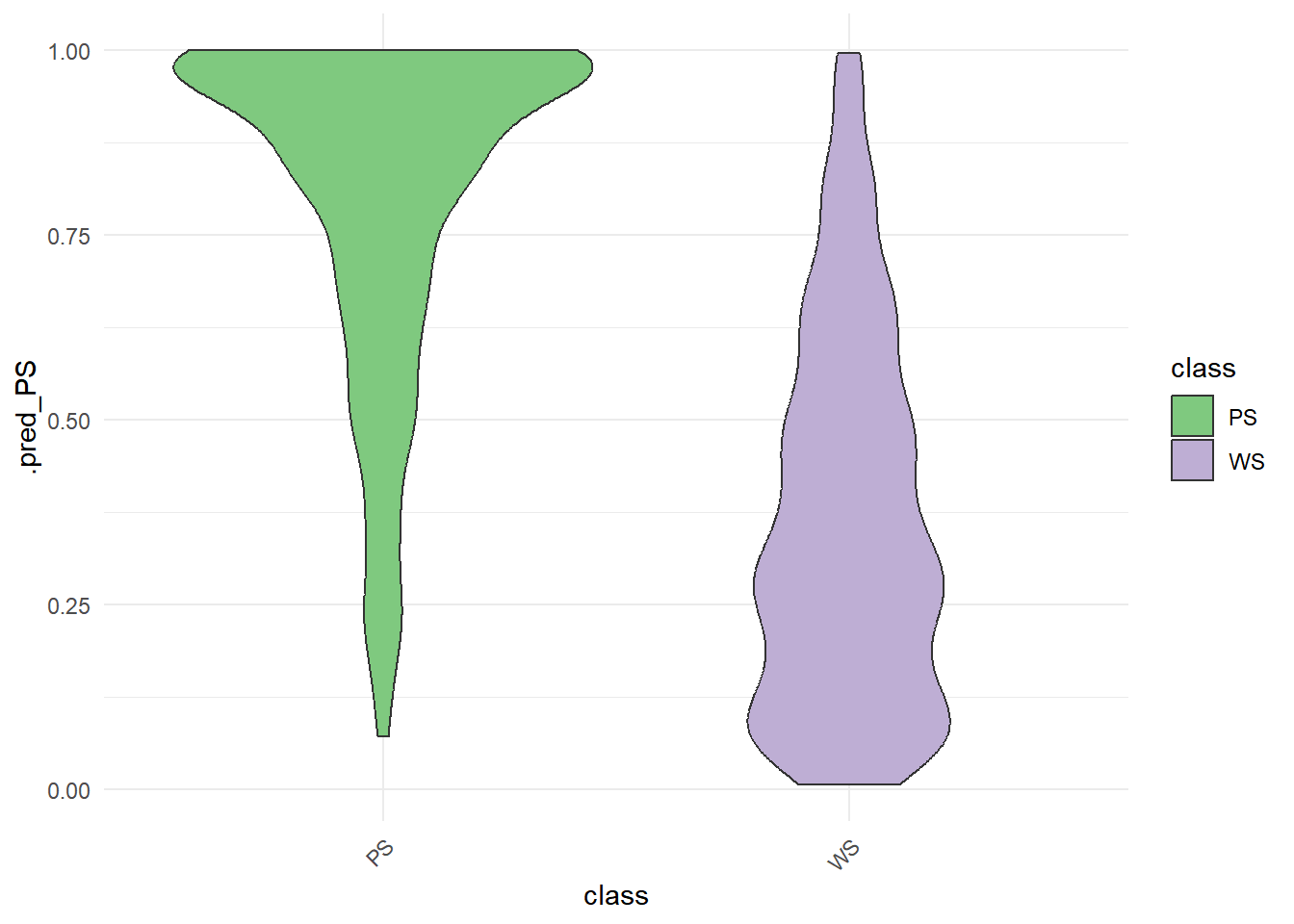
rf_testing_pred |>
  roc_curve(class, .pred_PS) |>
  autoplot()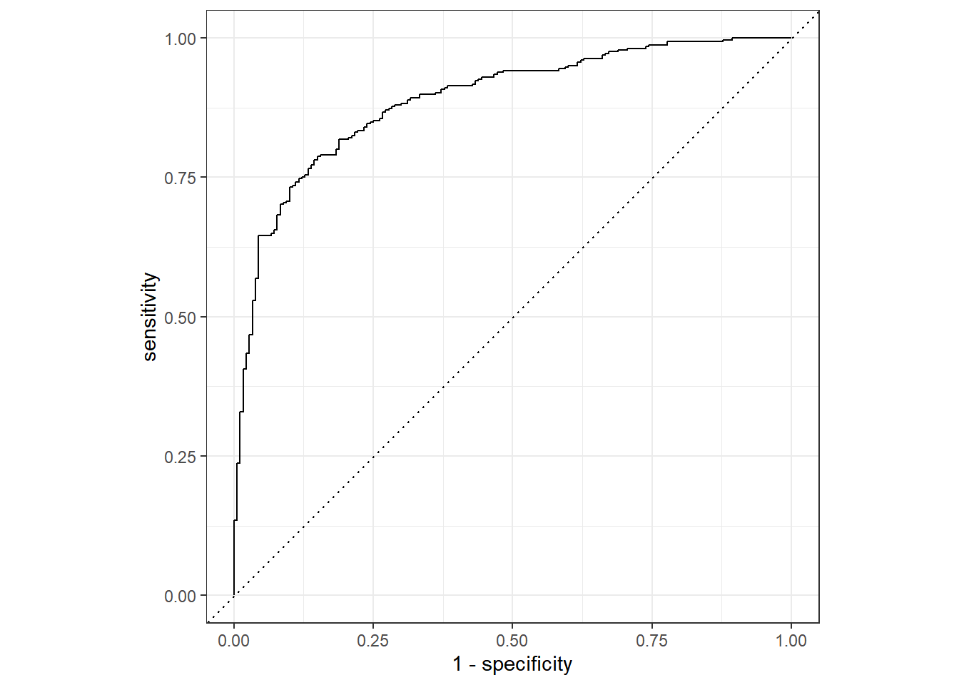
교차검증
그림에서처럼 Train Data를 쪼개서 각각을 다시 Trainin Set과 Testing Set으로 나누는 작업을 합니다. 예를 들어 현재 1514 개의 Traing Data의 Row 개수를 10개의 덩어리로 나눈다고 가정하겠습니다. 그럴 경우 90%의 데이터는 Analysis 데이터로 두고, 10%의 데이터를 Assessment 데이터로 두어서 모델을 적용하고 결과를 확인합니다. 결과를 낸 후 다른 그룹으로 90%와 10%를 각각 묶어 테스트합니다. 이렇게 10번의 과정을 겨치며 테스트 하는 것을 교차검증이라고 합니다.
###train 데이티를 10개의 묶음으로 랜덤하게 묶되, 그 아나에 train/test를 다시 나눈다.
set.seed(345)

folds <- vfold_cv(cell_train, v = 10)
folds
# 10-fold cross-validation
# A tibble: 10 × 2
splits id
<list> <chr>
1 <split [1362/152]> Fold01
2 <split [1362/152]> Fold02
3 <split [1362/152]> Fold03
4 <split [1362/152]> Fold04
5 <split [1363/151]> Fold05
6 <split [1363/151]> Fold06
7 <split [1363/151]> Fold07
8 <split [1363/151]> Fold08
9 <split [1363/151]> Fold09
10 <split [1363/151]> Fold10###v-fold 10개의 데이터셋에 랜덤포레스트 모델링을 하고 핏팅을 한다.
rf_wf <-
  workflow() %>%
  add_model(rf_mod) %>%
  add_formula(class ~ .)


set.seed(456)

rf_fit_rs <-
  rf_wf %>%
  fit_resamples(folds)
Warning: package 'ranger' was built under R version 4.3.2→ A | warning: 1000 columns were requested but there were 56 predictors in the data. 56 will be used.There were issues with some computations A: x1There were issues with some computations A: x2There were issues with some computations A: x3There were issues with some computations A: x4There were issues with some computations A: x5There were issues with some computations A: x6There were issues with some computations A: x7There were issues with some computations A: x8There were issues with some computations A: x9There were issues with some computations A: x10
There were issues with some computations A: x10###최종 성능 확인하기 (10개의 평균 accuracy, roc_auc)
collect_metrics(rf_fit_rs)# A tibble: 2 × 6
.metric .estimator mean n std_err .config
<chr> <chr> <dbl> <int> <dbl> <chr>
1 accuracy binary 0.817 10 0.00908 Preprocessor1_Model1
2 roc_auc binary 0.891 10 0.00692 Preprocessor1_Model1###의사결정나무 모델링할때 하이퍼파라미터 튜닝하기(트리깊이)
tune_spec <-
  decision_tree(
    cost_complexity = tune(),
    tree_depth = tune()
  ) %>%
  set_engine("rpart") %>%
  set_mode("classification")
###cost_complexity(5종류)와 트리깊이(5종류) 튜닝 - 25종류
tree_grid <- grid_regular(cost_complexity(),
                          tree_depth(),
                          levels = 5)

tree_grid
# A tibble: 25 × 2
cost_complexity tree_depth
<dbl> <int>
1 0.0000000001 1
2 0.0000000178 1
3 0.00000316 1
4 0.000562 1
5 0.1 1
6 0.0000000001 4
7 0.0000000178 4
8 0.00000316 4
9 0.000562 4
10 0.1 4
# ℹ 15 more rowstree_grid %>%
count(tree_depth)# A tibble: 5 × 2
tree_depth n
<int> <int>
1 1 5
2 4 5
3 8 5
4 11 5
5 15 5###25개의 트리모델을 이용하여 교차검증하기
set.seed(345)
cell_folds <- vfold_cv(cell_train, v = 10)


tree_wf <- workflow() %>%
  add_model(tune_spec) %>%
  add_formula(class ~ .)

tree_res <-
  tree_wf %>%
  tune_grid(
    resamples = cell_folds,
    grid = tree_grid
  )

tree_res
# Tuning results
# 10-fold cross-validation
# A tibble: 10 × 4
splits id .metrics .notes
<list> <chr> <list> <list>
1 <split [1362/152]> Fold01 <tibble [50 × 6]> <tibble [0 × 3]>
2 <split [1362/152]> Fold02 <tibble [50 × 6]> <tibble [0 × 3]>
3 <split [1362/152]> Fold03 <tibble [50 × 6]> <tibble [0 × 3]>
4 <split [1362/152]> Fold04 <tibble [50 × 6]> <tibble [0 × 3]>
5 <split [1363/151]> Fold05 <tibble [50 × 6]> <tibble [0 × 3]>
6 <split [1363/151]> Fold06 <tibble [50 × 6]> <tibble [0 × 3]>
7 <split [1363/151]> Fold07 <tibble [50 × 6]> <tibble [0 × 3]>
8 <split [1363/151]> Fold08 <tibble [50 × 6]> <tibble [0 × 3]>
9 <split [1363/151]> Fold09 <tibble [50 × 6]> <tibble [0 × 3]>
10 <split [1363/151]> Fold10 <tibble [50 × 6]> <tibble [0 × 3]>###교차검증 결과 보기
tree_res %>%
  collect_metrics()
# A tibble: 50 × 8
cost_complexity tree_depth .metric .estimator mean n std_err .config
<dbl> <int> <chr> <chr> <dbl> <int> <dbl> <chr>
1 0.0000000001 1 accuracy binary 0.733 10 0.00997 Preproces…
2 0.0000000001 1 roc_auc binary 0.778 10 0.00944 Preproces…
3 0.0000000178 1 accuracy binary 0.733 10 0.00997 Preproces…
4 0.0000000178 1 roc_auc binary 0.778 10 0.00944 Preproces…
5 0.00000316 1 accuracy binary 0.733 10 0.00997 Preproces…
6 0.00000316 1 roc_auc binary 0.778 10 0.00944 Preproces…
7 0.000562 1 accuracy binary 0.733 10 0.00997 Preproces…
8 0.000562 1 roc_auc binary 0.778 10 0.00944 Preproces…
9 0.1 1 accuracy binary 0.733 10 0.00997 Preproces…
10 0.1 1 roc_auc binary 0.778 10 0.00944 Preproces…
# ℹ 40 more rows###복잡도와 트리깊이 5종류에 대해 각각의 accuracy와 roc_auc 보기
tree_res %>%
  collect_metrics() %>%
  # tree depth를 factor로 치환
  mutate(tree_depth = factor(tree_depth)) %>%
  ggplot(aes(cost_complexity, mean, color = tree_depth))+
  geom_line(alpha = 0.6)+
  geom_point(size = 2)+
  # metric을 차원으로 그래프를 두 개로 나눔
  facet_wrap( ~ .metric, scales = 'free', nrow = 2)+
  # log scale을 적용
  scale_x_log10(labels = scales::label_number()) # Decimal Format으로 강제함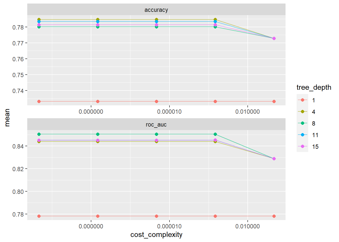
###가장 좋은 모델 선택하기 (show_best()), 기준은 roc_auc
 tree_res %>%
  show_best("roc_auc")
# A tibble: 5 × 8
cost_complexity tree_depth .metric .estimator mean n std_err .config
<dbl> <int> <chr> <chr> <dbl> <int> <dbl> <chr>
1 0.0000000001 8 roc_auc binary 0.850 10 0.00729 Preprocesso…
2 0.0000000178 8 roc_auc binary 0.850 10 0.00729 Preprocesso…
3 0.00000316 8 roc_auc binary 0.850 10 0.00729 Preprocesso…
4 0.000562 8 roc_auc binary 0.850 10 0.00729 Preprocesso…
5 0.000562 11 roc_auc binary 0.845 10 0.00706 Preprocesso…best_tree <- tree_res %>%
select_best("roc_auc")
best_tree# A tibble: 1 × 3
cost_complexity tree_depth .config
<dbl> <int> <chr>
1 0.0000000001 8 Preprocessor1_Model11###best 모델로 모델링하기
final_wf <-
  tree_wf %>%
  finalize_workflow(best_tree)

final_wf
══ Workflow ════════════════════════════════════════════════════════════════════
Preprocessor: Formula
Model: decision_tree()
── Preprocessor ────────────────────────────────────────────────────────────────
class ~ .
── Model ───────────────────────────────────────────────────────────────────────
Decision Tree Model Specification (classification)
Main Arguments:
cost_complexity = 1e-10
tree_depth = 8
Computational engine: rpart ###훈련데이터를 넣어 best 모델링하기
final_tree <-
  final_wf %>%
  fit(data = cell_train)

final_wf
══ Workflow ════════════════════════════════════════════════════════════════════
Preprocessor: Formula
Model: decision_tree()
── Preprocessor ────────────────────────────────────────────────────────────────
class ~ .
── Model ───────────────────────────────────────────────────────────────────────
Decision Tree Model Specification (classification)
Main Arguments:
cost_complexity = 1e-10
tree_depth = 8
Computational engine: rpart ###변수별 중요도 보기
library(vip)Warning: package 'vip' was built under R version 4.3.2
Attaching package: 'vip'The following object is masked from 'package:utils':
vifinal_tree %>%
pull_workflow_fit() %>%
vip()Warning: `pull_workflow_fit()` was deprecated in workflows 0.2.3.
ℹ Please use `extract_fit_parsnip()` instead.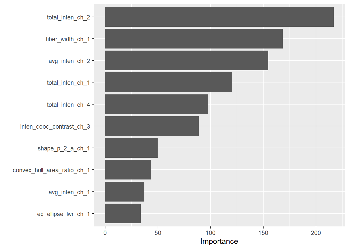
###best 모델로 test 데이터 넣고 예측하기
final_fit <-
  final_wf %>%
  # recipe로 나누었던 cell_split에 대하여 Last_fit함수 적용
  last_fit(cells_split)

final_fit %>%
  collect_metrics()
# A tibble: 2 × 4
.metric .estimator .estimate .config
<chr> <chr> <dbl> <chr>
1 accuracy binary 0.772 Preprocessor1_Model1
2 roc_auc binary 0.847 Preprocessor1_Model1###roc-curve보기
final_fit %>%
  # 예측결과 도출
  collect_predictions() %>%
  # ROC Cure 도출
  roc_curve(class, .pred_PS) %>%
  # Plot 그리기
  autoplot()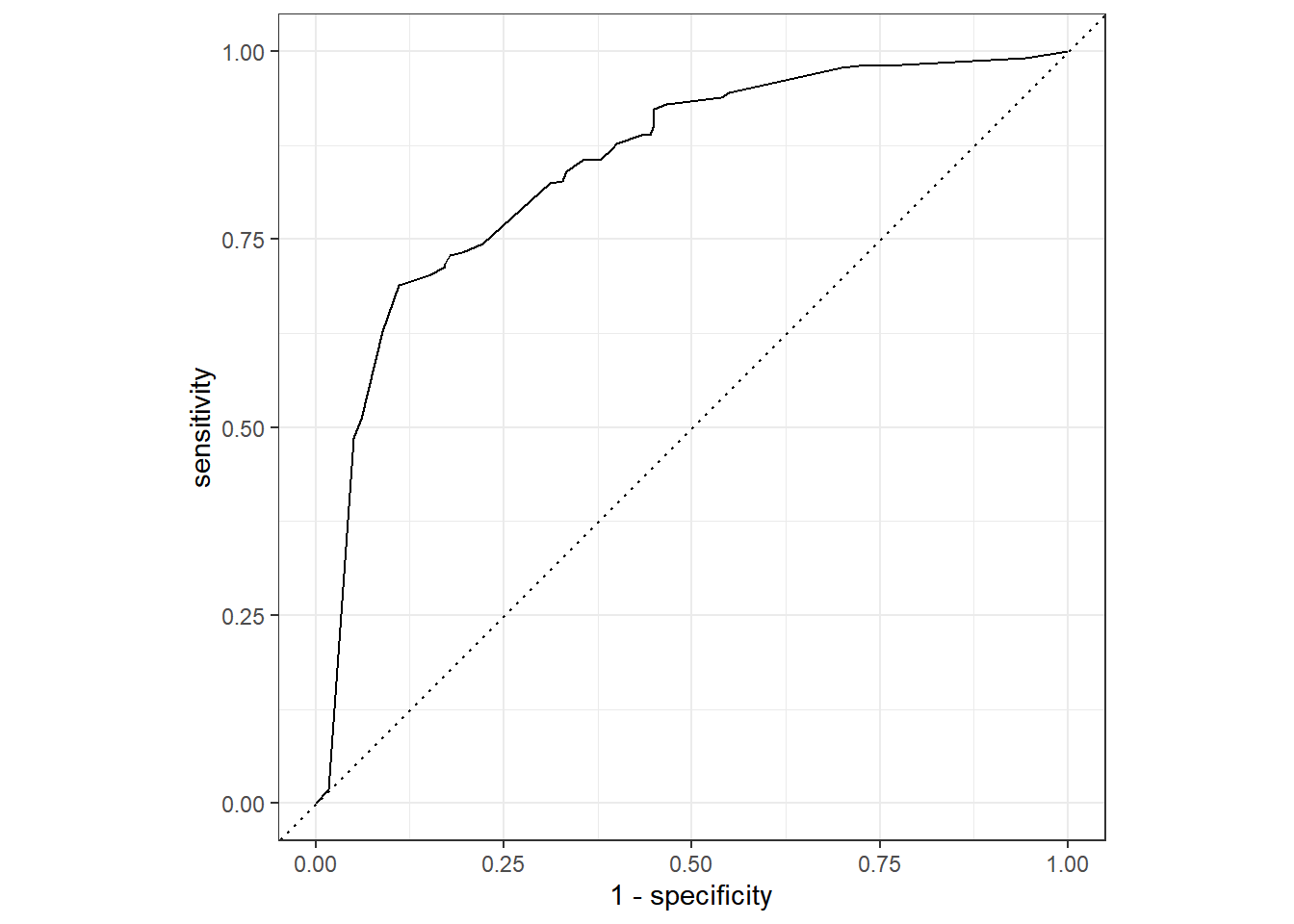
##노모그램 그리기
관련논문
if(!require('rms')) {
  install.packages('rms')
  library('rms')
}
Loading required package: rmsWarning: package 'rms' was built under R version 4.3.2Loading required package: HmiscWarning: package 'Hmisc' was built under R version 4.3.2
Attaching package: 'Hmisc'The following object is masked from 'package:parsnip':
translateThe following objects are masked from 'package:dplyr':
src, summarizeThe following objects are masked from 'package:base':
format.pval, unitsWarning in .recacheSubclasses(def@className, def, env): undefined subclass
"ndiMatrix" of class "replValueSp"; definition not updatedn <- 1000 # define sample size
set.seed(17) # so can reproduce the results
d <- data.frame(age = rnorm(n, 50, 10),
blood.pressure = rnorm(n, 120, 15),
cholesterol = rnorm(n, 200, 25),
sex = factor(sample(c('female','male'), n,TRUE)))
# Specify population model for log odds that Y=1
# Simulate binary y to have Prob(y=1) = 1/[1+exp(-L)]
d <- upData(d,
L = .4*(sex=='male') + .045*(age-50) +
(log(cholesterol - 10)-5.2)*(-2*(sex=='female') + 2*(sex=='male')),
y = ifelse(runif(n) < plogis(L), 1, 0))Input object size: 29616 bytes; 4 variables 1000 observations
Added variable L
Added variable y
New object size: 41856 bytes; 6 variables 1000 observationsddist <- datadist(d); options(datadist='ddist')
f <- lrm(y ~ lsp(age,50) + sex * rcs(cholesterol, 4) + blood.pressure,
data=d)
nom <- nomogram(f, fun=function(x)1/(1+exp(-x)), # or fun=plogis
fun.at=c(.001,.01,.05,seq(.1,.9,by=.1),.95,.99,.999),
funlabel="Risk of Death")
#Instead of fun.at, could have specified fun.lp.at=logit of
#sequence above - faster and slightly more accurate
plot(nom, xfrac=.45)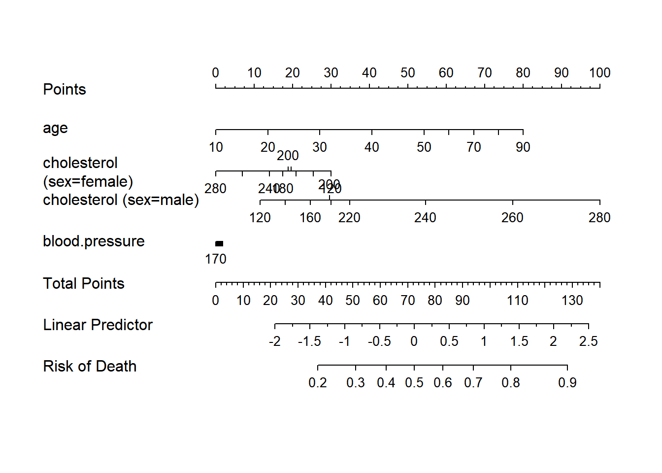
print(nom)Points per unit of linear predictor: 25.39362
Linear predictor units per point : 0.03937996
age Points
10 0
20 14
30 27
40 41
50 54
60 61
70 67
80 74
90 80
cholesterol (sex=female) Points
120 30
140 25
160 21
180 17
200 19
220 20
240 14
260 7
280 0
cholesterol (sex=male) Points
120 12
140 18
160 25
180 30
200 30
220 35
240 55
260 77
280 100
blood.pressure Points
70 2
80 2
90 1
100 1
110 1
120 1
130 1
140 1
150 0
160 0
170 0
Total Points Risk of Death
37 0.2
51 0.3
62 0.4
72 0.5
83 0.6
94 0.7
108 0.8
128 0.9nom <- nomogram(f, age=seq(10,90,by=10))
plot(nom, xfrac=.45)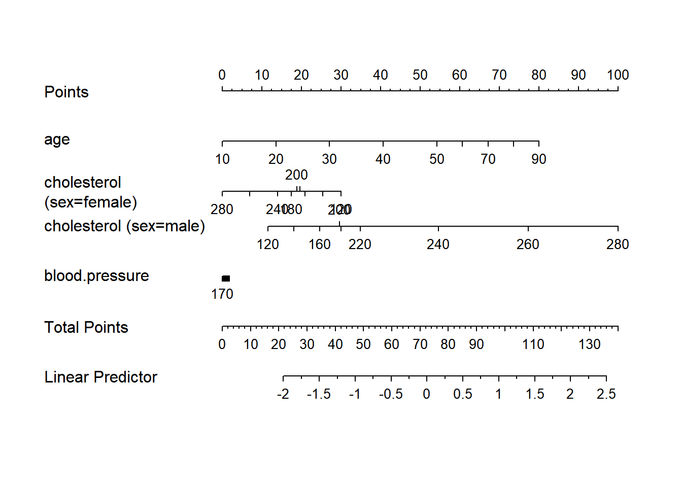
g <- lrm(y ~ sex + rcs(age, 3) * rcs(cholesterol, 3), data=d)
nom <- nomogram(g, interact=list(age=c(20,40,60)),
                conf.int=c(.7,.9,.95))
plot(nom, col.conf=c(1,.5,.2), naxes=7)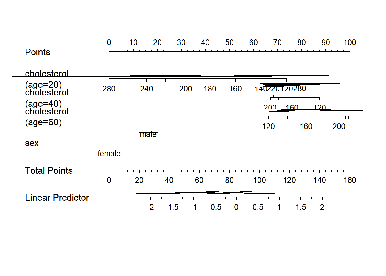
require(survival)Loading required package: survivalWarning: package 'survival' was built under R version 4.3.2w <- upData(d,
cens = 15 * runif(n),
h = .02 * exp(.04 * (age - 50) + .8 * (sex == 'Female')),
d.time = -log(runif(n)) / h,
death = ifelse(d.time <= cens, 1, 0),
d.time = pmin(d.time, cens))Input object size: 41856 bytes; 6 variables 1000 observations
Added variable cens
Added variable h
Added variable d.time
Added variable death
Modified variable d.time
New object size: 70432 bytes; 10 variables 1000 observationsf <- psm(Surv(d.time,death) ~ sex * age, data=w, dist='lognormal')
med <- Quantile(f)
surv <- Survival(f) # This would also work if f was from cph
plot(nomogram(f, fun=function(x) med(lp=x), funlabel="Median Survival Time"))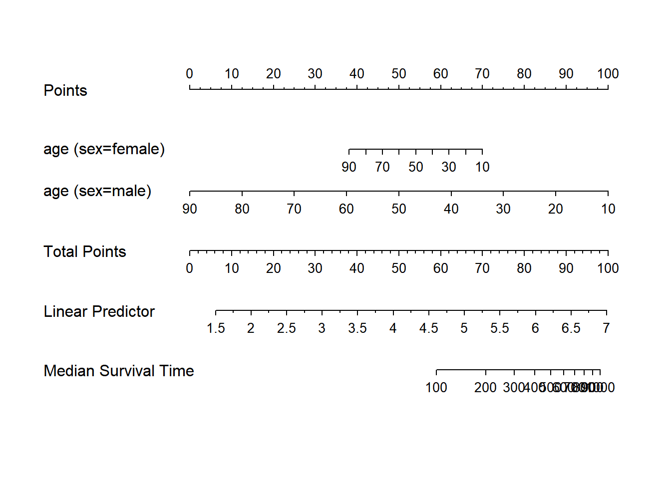
nom <- nomogram(f, fun=list(function(x) surv(3, x),
                            function(x) surv(6, x)),
                funlabel=c("3-Month Survival Probability",
                           "6-month Survival Probability"))
plot(nom, xfrac=.7)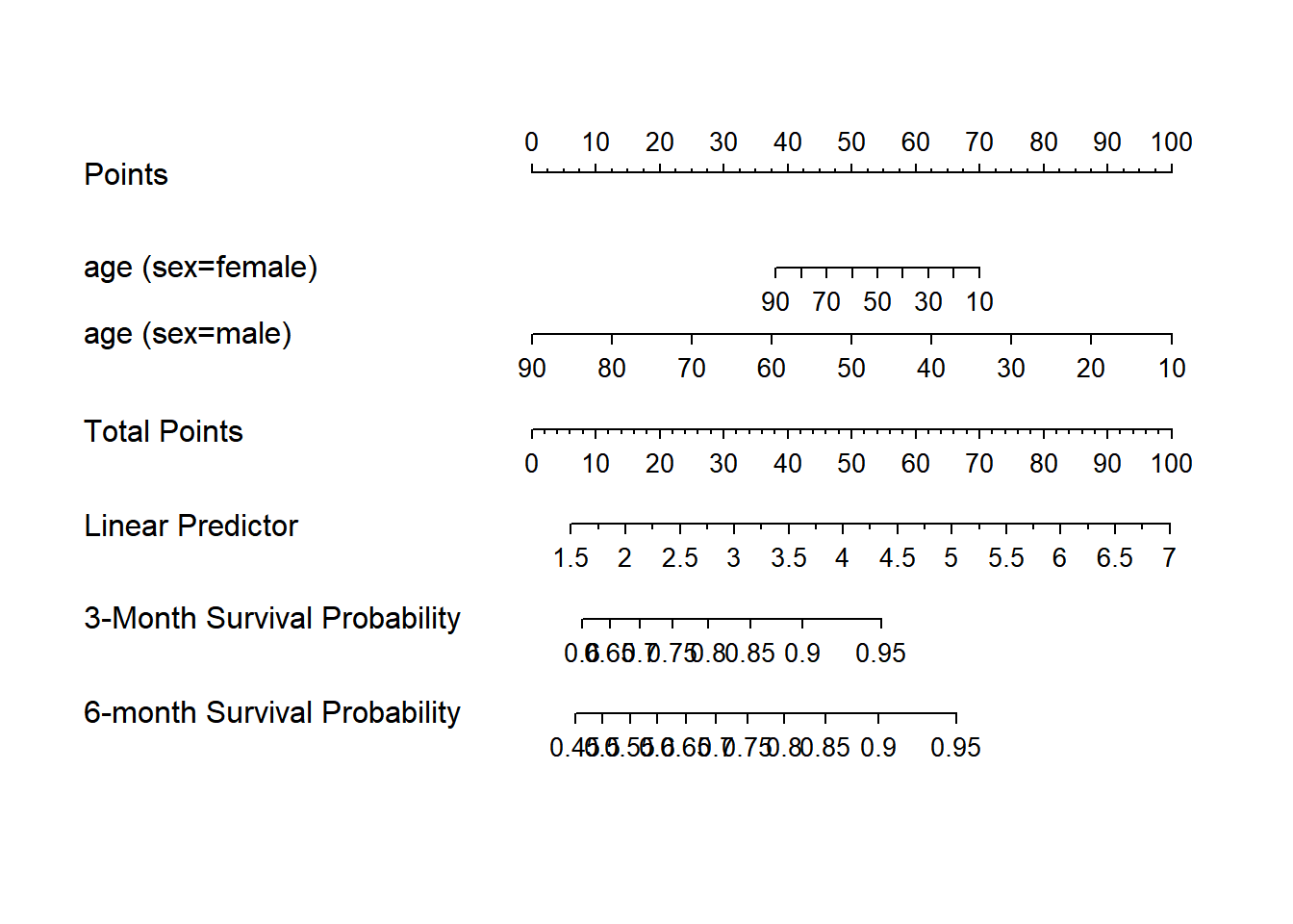
if (FALSE) {
  nom <- nomogram(fit.with.categorical.predictors, abbrev=TRUE, minlength=1)
  nom$x1$points   # print points assigned to each level of x1 for its axis
  #Add legend for abbreviations for category levels
  abb <- attr(nom, 'info')$abbrev$treatment
  legend(locator(1), abb$full, pch=paste(abb$abbrev,collapse=''),
         ncol=2, bty='n')  # this only works for 1-letter abbreviations
  #Or use the legend.nomabbrev function:
  legend.nomabbrev(nom, 'treatment', locator(1), ncol=2, bty='n')
}


#Make a nomogram with axes predicting probabilities Y>=j for all j=1-3
#in an ordinal logistic model, where Y=0,1,2,3
w <- upData(w, Y = ifelse(y==0, 0, sample(1:3, length(y), TRUE)))
Input object size: 70432 bytes; 10 variables 1000 observations
Added variable Y
New object size: 74536 bytes; 11 variables 1000 observationsg <- lrm(Y ~ age+rcs(cholesterol,4) * sex, data=w)
fun2 <- function(x) plogis(x-g$coef[1]+g$coef[2])
fun3 <- function(x) plogis(x-g$coef[1]+g$coef[3])
f <- Newlabels(g, c(age='Age in Years'))
#see Design.Misc, which also has Newlevels to change
#labels for levels of categorical variables
g <- nomogram(f, fun=list('Prob Y>=1'=plogis, 'Prob Y>=2'=fun2,
'Prob Y=3'=fun3),
fun.at=c(.01,.05,seq(.1,.9,by=.1),.95,.99))
plot(g, lmgp=.2, cex.axis=.6)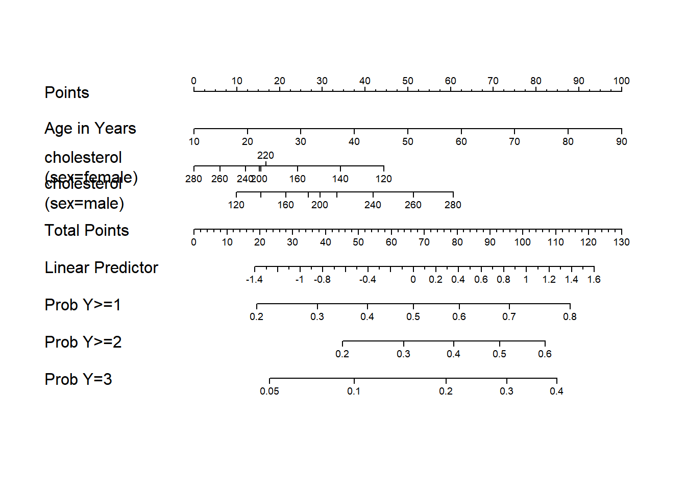
options(datadist=NULL)library(stargazer)
## Latex 형태 테이블
stargazer(mtcars, type= "text", title= "Summary Statistics", out= "mtcars.text")
Summary Statistics
============================================
Statistic N   Mean   St. Dev.  Min     Max
--------------------------------------------
mpg       32 20.091   6.027   10.400 33.900
cyl       32  6.188   1.786     4       8
disp      32 230.722 123.939  71.100 472.000
hp        32 146.688  68.563    52     335
drat      32  3.597   0.535   2.760   4.930
wt        32  3.217   0.978   1.513   5.424
qsec      32 17.849   1.787   14.500 22.900
vs        32  0.438   0.504     0       1
am        32  0.406   0.499     0       1
gear      32  3.688   0.738     3       5
carb      32  2.812   1.615     1       8
--------------------------------------------
## apply a list of functions to a list or vector
f <- function(X, FUN, ...) {
fn <- as.character(match.call()$FUN)[-1]
out <- sapply(FUN, mapply, X, ...)
setNames(as.data.frame(out), fn)
}
(out <- round(f(attitude, list(mean, sd, median, min, max)), 2)) mean sd median min max
rating 64.63 12.17 65.5 40 85
complaints 66.60 13.31 65.0 37 90
privileges 53.13 12.24 51.5 30 83
learning 56.37 11.74 56.5 34 75
raises 64.63 10.40 63.5 43 88
critical 74.77 9.89 77.5 49 92
advance 42.93 10.29 41.0 25 72library('htmlTable')Warning: package 'htmlTable' was built under R version 4.3.2htmlTable(out, cgroup = 'Statistic', n.cgroup = 5, caption = 'Table 1: default')| Table 1: default | |||||
|---|---|---|---|---|---|
| Statistic | |||||
| mean | sd | median | min | max | |
| rating | 64.63 | 12.17 | 65.5 | 40 | 85 |
| complaints | 66.6 | 13.31 | 65 | 37 | 90 |
| privileges | 53.13 | 12.24 | 51.5 | 30 | 83 |
| learning | 56.37 | 11.74 | 56.5 | 34 | 75 |
| raises | 64.63 | 10.4 | 63.5 | 43 | 88 |
| critical | 74.77 | 9.89 | 77.5 | 49 | 92 |
| advance | 42.93 | 10.29 | 41 | 25 | 72 |
htmlTable(out, cgroup = 'Statistic', n.cgroup = 5, caption = 'Table 1: padding',
          ## padding to cells: top side bottom
css.cell = 'padding: 0px 10px 0px;')| Table 1: padding | |||||
|---|---|---|---|---|---|
| Statistic | |||||
| mean | sd | median | min | max | |
| rating | 64.63 | 12.17 | 65.5 | 40 | 85 |
| complaints | 66.6 | 13.31 | 65 | 37 | 90 |
| privileges | 53.13 | 12.24 | 51.5 | 30 | 83 |
| learning | 56.37 | 11.74 | 56.5 | 34 | 75 |
| raises | 64.63 | 10.4 | 63.5 | 43 | 88 |
| critical | 74.77 | 9.89 | 77.5 | 49 | 92 |
| advance | 42.93 | 10.29 | 41 | 25 | 72 |
문건웅 교수 패키지
테이블
#install.packages("moonBook")
library(moonBook)
Warning: package 'moonBook' was built under R version 4.3.2
Attaching package: 'moonBook'The following object is masked from 'package:scales':
commadata(acs)
mytable(sex~age+Dx, data=acs)
         Descriptive Statistics by 'sex'
——————————————————————————————————————————————————
                       Female       Male       p
                       (N=287)     (N=570)
——————————————————————————————————————————————————
 age                 68.7 ± 10.7 60.6 ± 11.2 0.000
 Dx                                          0.012
   - NSTEMI          50 (17.4%)  103 (18.1%)
   - STEMI           84 (29.3%)  220 (38.6%)
   - Unstable Angina 153 (53.3%) 247 (43.3%)
——————————————————————————————————————————————————
테이블 만들기
str(mtcars)'data.frame': 32 obs. of 11 variables:
$ mpg : num 21 21 22.8 21.4 18.7 18.1 14.3 24.4 22.8 19.2 ...
$ cyl : num 6 6 4 6 8 6 8 4 4 6 ...
$ disp: num 160 160 108 258 360 ...
$ hp : num 110 110 93 110 175 105 245 62 95 123 ...
$ drat: num 3.9 3.9 3.85 3.08 3.15 2.76 3.21 3.69 3.92 3.92 ...
$ wt : num 2.62 2.88 2.32 3.21 3.44 ...
$ qsec: num 16.5 17 18.6 19.4 17 ...
$ vs : num 0 0 1 1 0 1 0 1 1 1 ...
$ am : num 1 1 1 0 0 0 0 0 0 0 ...
$ gear: num 4 4 4 3 3 3 3 4 4 4 ...
$ carb: num 4 4 1 1 2 1 4 2 2 4 ...#mytable 함수에서는 고유값이 5개 미만인 경우 숫자로 입력되어 있더라도 연속형 변수가 아닌 범주형 변수로 취급합니다.
mytable(am~., data=mtcars)
    Descriptive Statistics by 'am'
———————————————————————————————————————
             0            1         p
          (N=19)        (N=13)
———————————————————————————————————————
 mpg    17.1 ±  3.8  24.4 ±  6.2  0.000
 cyl                              0.013
   - 4   3 (15.8%)    8 (61.5%)
   - 6   4 (21.1%)    3 (23.1%)
   - 8  12 (63.2%)    2 (15.4%)
 disp  290.4 ± 110.2 143.5 ± 87.2 0.000
 hp    160.3 ± 53.9  126.8 ± 84.1 0.180
 drat    3.3 ±  0.4   4.0 ±  0.4  0.000
 wt      3.8 ±  0.8   2.4 ±  0.6  0.000
 qsec   18.2 ±  1.8  17.4 ±  1.8  0.206
 vs                               0.556
   - 0  12 (63.2%)    6 (46.2%)
   - 1   7 (36.8%)    7 (53.8%)
 gear                             0.000
   - 3  15 (78.9%)     0 ( 0.0%)
   - 4   4 (21.1%)    8 (61.5%)
   - 5   0 ( 0.0%)    5 (38.5%)
 carb    2.7 ±  1.1   2.9 ±  2.2  0.781
———————————————————————————————————————
#carb 범주형 변수로 취급하고 싶다면 [max.ylev]의 인수를 바꿔주면 됩니다.
mytable(am~carb, data=mtcars,max.ylev=6)
  Descriptive Statistics by 'am'
——————————————————————————————————
           0          1        p
         (N=19)     (N=13)
——————————————————————————————————
 carb                        0.284
   - 1 3 (15.8%)  4 (30.8%)
   - 2 6 (31.6%)  4 (30.8%)
   - 3 3 (15.8%)   0 ( 0.0%)
   - 4 7 (36.8%)  3 (23.1%)
   - 6  0 ( 0.0%) 1 ( 7.7%)
   - 8  0 ( 0.0%) 1 ( 7.7%)
——————————————————————————————————
###1.4 여러개의 표를 하나로 합치기
# 전체 환자를 성별에 따라 남, 여로 나누고 다시 당뇨병 유무에 따라 표를 나누어 만든 후 표를 합치고 싶으면 다음과 같이 합니다.
mytable(sex+DM~., data=acs)
                 Descriptive Statistics stratified by 'sex' and 'DM'
—————————————————————————————————————————————————————————————————————————————————————
                                    Male                             Female
                     ———————————————————————————————— ———————————————————————————————
                          No           Yes        p        No          Yes        p
                       (N=380)       (N=190)           (N=173)      (N=114)
—————————————————————————————————————————————————————————————————————————————————————
 age                 60.9 ± 11.5   60.1 ± 10.6  0.472 69.3 ± 11.4  67.8 ±  9.7  0.257
 cardiogenicShock                               0.685                           0.296
   - No              355 (93.4%)   175 (92.1%)        168 (97.1%)  107 (93.9%)
   - Yes              25 ( 6.6%)   15 ( 7.9%)          5 ( 2.9%)    7 ( 6.1%)
 entry                                          0.552                           0.665
   - Femoral         125 (32.9%)   68 (35.8%)          74 (42.8%)   45 (39.5%)
   - Radial          255 (67.1%)   122 (64.2%)         99 (57.2%)   69 (60.5%)
 Dx                                             0.219                           0.240
   - NSTEMI           71 (18.7%)   32 (16.8%)          25 (14.5%)   25 (21.9%)
   - STEMI           154 (40.5%)   66 (34.7%)          54 (31.2%)   30 (26.3%)
   - Unstable Angina 155 (40.8%)   92 (48.4%)          94 (54.3%)   59 (51.8%)
 EF                  56.5 ±  8.3   53.9 ± 11.0  0.007 56.0 ± 10.1  56.6 ± 10.0  0.655
 height              168.1 ±  5.8 167.5 ±  6.7  0.386 153.9 ±  6.5 153.6 ±  5.8 0.707
 weight              68.1 ± 10.4   69.8 ± 10.2  0.070 56.5 ±  8.7  58.4 ± 10.0  0.106
 BMI                 24.0 ±  3.1   24.9 ±  3.5  0.005 23.8 ±  3.2  24.8 ±  4.0  0.046
 obesity                                        0.027                           0.359
   - No              261 (68.7%)   112 (58.9%)        121 (69.9%)   73 (64.0%)
   - Yes             119 (31.3%)   78 (41.1%)          52 (30.1%)   41 (36.0%)
 TC                  184.1 ± 46.7 181.8 ± 44.5  0.572 186.0 ± 43.1 193.3 ± 60.8 0.274
 LDLC                117.9 ± 41.8 112.1 ± 39.4  0.115 116.3 ± 35.2 119.8 ± 48.6 0.519
 HDLC                38.4 ± 11.4   36.8 ±  9.6  0.083 39.2 ± 10.9  38.8 ± 12.2  0.821
 TG                  115.2 ± 72.2 153.4 ± 130.7 0.000 114.2 ± 82.4 128.4 ± 65.5 0.112
 HBP                                            0.000                           0.356
   - No              205 (53.9%)   68 (35.8%)          54 (31.2%)   29 (25.4%)
   - Yes             175 (46.1%)   122 (64.2%)        119 (68.8%)   85 (74.6%)
 smoking                                        0.386                           0.093
   - Ex-smoker       101 (26.6%)   54 (28.4%)          34 (19.7%)   15 (13.2%)
   - Never            77 (20.3%)   46 (24.2%)         118 (68.2%)   91 (79.8%)
   - Smoker          202 (53.2%)   90 (47.4%)          21 (12.1%)   8 ( 7.0%)
—————————————————————————————————————————————————————————————————————————————————————
#1.5 csv 파일로 저장하기
mycsv(mytable(sex+DM~., data=acs),file='test1.csv')
mycsv(mytable(sex+DM~age+Dx, data=acs),file='test2.csv')
#1.6 html 형식으로 표를 출력하기
# myhtml(mytable(sex+DM~., data=acs))
# myhtml(mytable(sex+DM~age+Dx, data=acs))히스토그램
require(UsingR)Loading required package: UsingRWarning: package 'UsingR' was built under R version 4.3.2Loading required package: MASS
Attaching package: 'MASS'The following object is masked from 'package:dplyr':
selectLoading required package: HistDataWarning: package 'HistData' was built under R version 4.3.2
Attaching package: 'UsingR'The following object is masked from 'package:survival':
cancerdata(galton)
str(galton)'data.frame': 928 obs. of 2 variables:
$ child : num 61.7 61.7 61.7 61.7 61.7 62.2 62.2 62.2 62.2 62.2 ...
$ parent: num 70.5 68.5 65.5 64.5 64 67.5 67.5 67.5 66.5 66.5 ...par(mfrow=c(1,2))
hist(galton$child, col="blue", breaks = 100)
hist(galton$parent, col="blue", breaks = 100)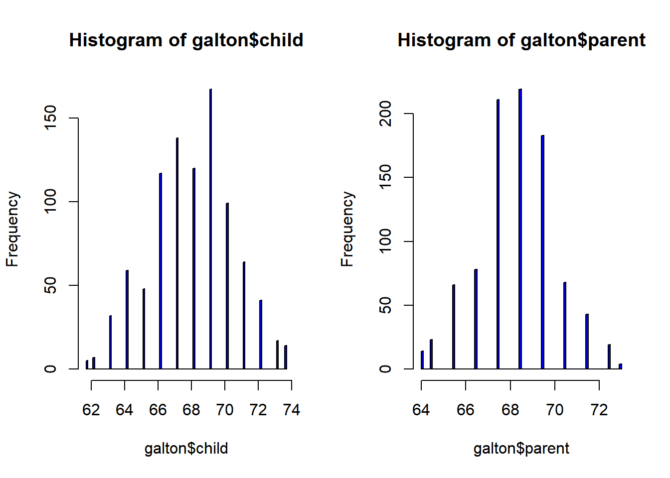
##상관관계
par(mfrow=c(1,1)) # Default
cor.test(galton$child, galton$parent)
    Pearson's product-moment correlation

data:  galton$child and galton$parent
t = 15.711, df = 926, p-value < 2.2e-16
alternative hypothesis: true correlation is not equal to 0
95 percent confidence interval:
 0.4064067 0.5081153
sample estimates:
      cor
0.4587624
#부모와 아이 키 상관표
xtabs(~child+parent, data=galton) parent
child 64 64.5 65.5 66.5 67.5 68.5 69.5 70.5 71.5 72.5 73
61.7 1 1 1 0 0 1 0 1 0 0 0
62.2 0 1 0 3 3 0 0 0 0 0 0
63.2 2 4 9 3 5 7 1 1 0 0 0
64.2 4 4 5 5 14 11 16 0 0 0 0
65.2 1 1 7 2 15 16 4 1 1 0 0
66.2 2 5 11 17 36 25 17 1 3 0 0
67.2 2 5 11 17 38 31 27 3 4 0 0
68.2 1 0 7 14 28 34 20 12 3 1 0
69.2 1 2 7 13 38 48 33 18 5 2 0
70.2 0 0 5 4 19 21 25 14 10 1 0
71.2 0 0 2 0 11 18 20 7 4 2 0
72.2 0 0 1 0 4 4 11 4 9 7 1
73.2 0 0 0 0 0 3 4 3 2 2 3
73.7 0 0 0 0 0 0 5 3 2 4 0##회귀분석
out = lm(child~parent, data=galton)
summary(out)
Call:
lm(formula = child ~ parent, data = galton)

Residuals:
    Min      1Q  Median      3Q     Max
-7.8050 -1.3661  0.0487  1.6339  5.9264

Coefficients:
            Estimate Std. Error t value Pr(>|t|)
(Intercept) 23.94153    2.81088   8.517   <2e-16 ***
parent       0.64629    0.04114  15.711   <2e-16 ***
---
Signif. codes:  0 '***' 0.001 '**' 0.01 '*' 0.05 '.' 0.1 ' ' 1

Residual standard error: 2.239 on 926 degrees of freedom
Multiple R-squared:  0.2105,    Adjusted R-squared:  0.2096
F-statistic: 246.8 on 1 and 926 DF, p-value: < 2.2e-16plot(child~parent, data=galton)
abline(out,col='red')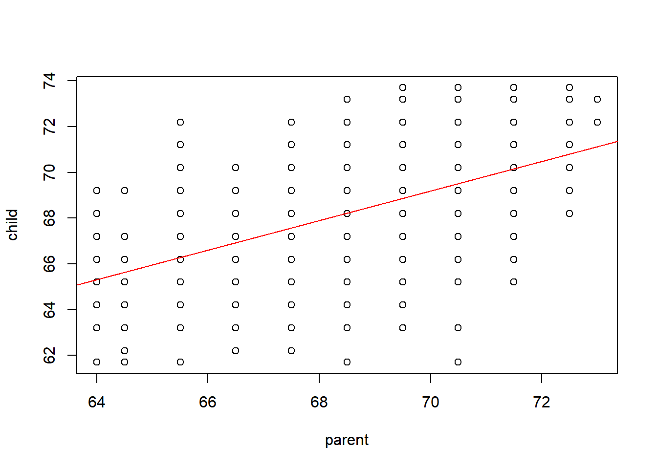
## 단순회귀 분석
data(women)
str(women)
'data.frame': 15 obs. of 2 variables:
$ height: num 58 59 60 61 62 63 64 65 66 67 ...
$ weight: num 115 117 120 123 126 129 132 135 139 142 ...fit = lm(weight~height, data=women)
summary(fit)
Call:
lm(formula = weight ~ height, data = women)

Residuals:
    Min      1Q  Median      3Q     Max
-1.7333 -1.1333 -0.3833  0.7417  3.1167

Coefficients:
             Estimate Std. Error t value Pr(>|t|)
(Intercept) -87.51667    5.93694  -14.74 1.71e-09 ***
height        3.45000    0.09114   37.85 1.09e-14 ***
---
Signif. codes:  0 '***' 0.001 '**' 0.01 '*' 0.05 '.' 0.1 ' ' 1

Residual standard error: 1.525 on 13 degrees of freedom
Multiple R-squared:  0.991, Adjusted R-squared:  0.9903
F-statistic: 1433 on 1 and 13 DF, p-value: 1.091e-14plot(weight~height, data=women)
abline(fit, col='blue')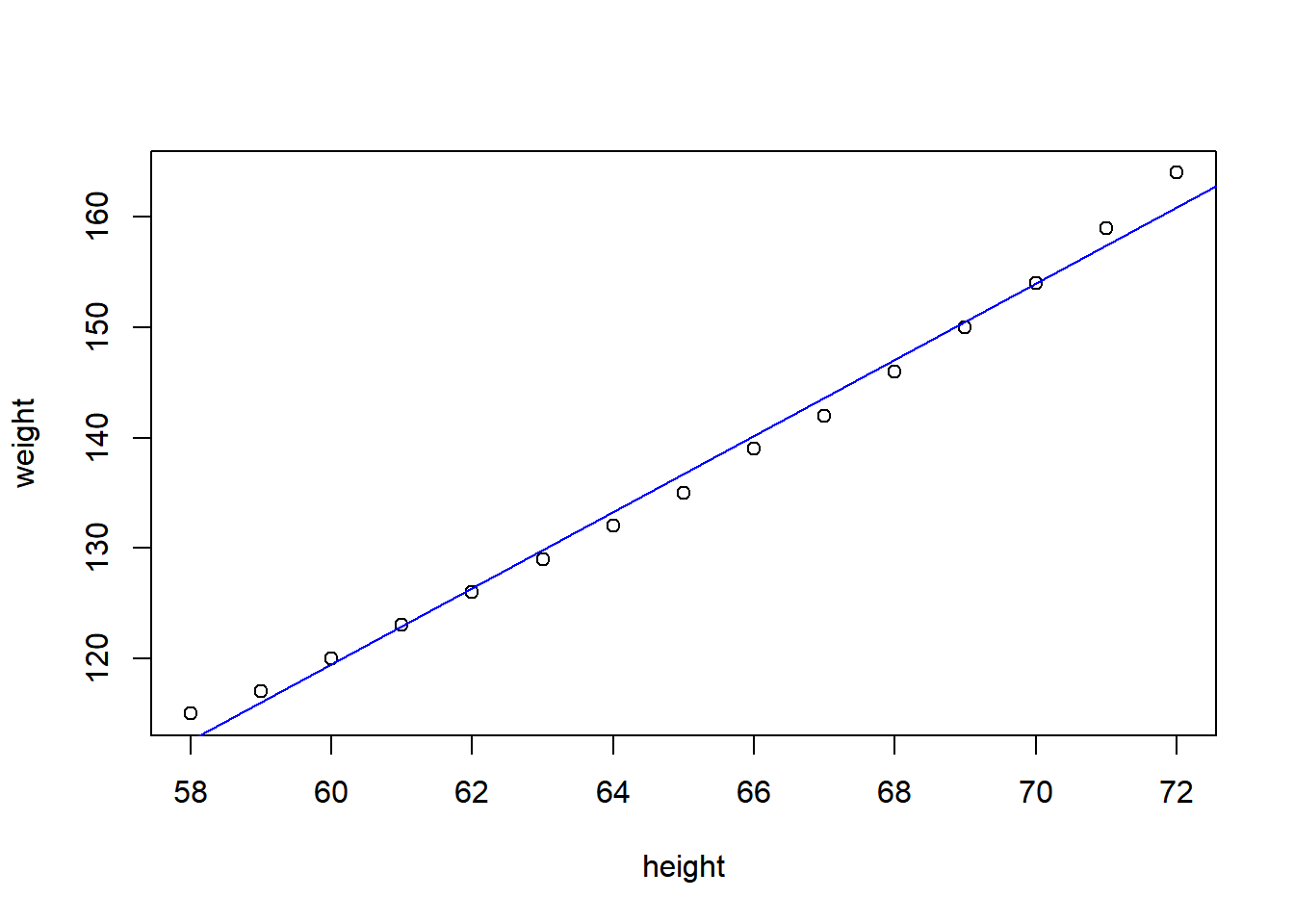
fit2 = lm(weight~height+I(height^2), data=women)
summary(fit2)
Call:
lm(formula = weight ~ height + I(height^2), data = women)

Residuals:
     Min       1Q   Median       3Q      Max
-0.50941 -0.29611 -0.00941  0.28615  0.59706

Coefficients:
             Estimate Std. Error t value Pr(>|t|)
(Intercept) 261.87818   25.19677  10.393 2.36e-07 ***
height       -7.34832    0.77769  -9.449 6.58e-07 ***
I(height^2)   0.08306    0.00598  13.891 9.32e-09 ***
---
Signif. codes:  0 '***' 0.001 '**' 0.01 '*' 0.05 '.' 0.1 ' ' 1

Residual standard error: 0.3841 on 12 degrees of freedom
Multiple R-squared:  0.9995,    Adjusted R-squared:  0.9994
F-statistic: 1.139e+04 on 2 and 12 DF, p-value: < 2.2e-16plot(weight~height,data=women)
lines(women$height, fitted(fit2), col="red")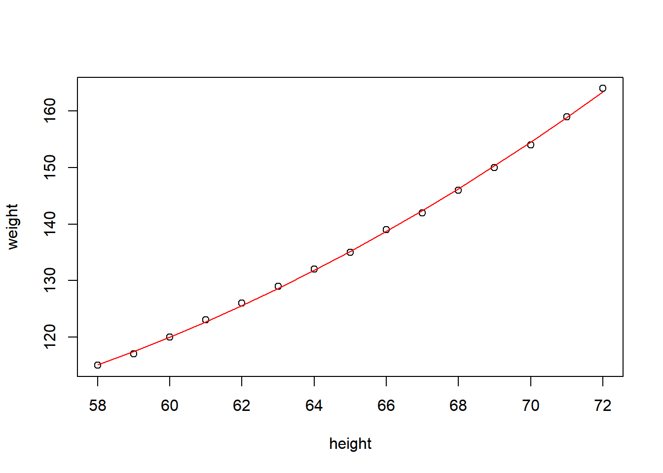
scatterplot
require(car)Loading required package: carLoading required package: carData
Attaching package: 'car'The following objects are masked from 'package:rms':
Predict, vifThe following object is masked from 'package:dplyr':
recodeThe following object is masked from 'package:purrr':
somescatterplot(weight~height, data=women)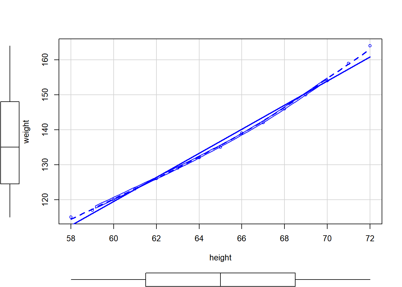
scatterplot(weight~height, data=women, pch=19, # pch=점을 속이 차있는 circle
            spread=FALSE, smoother.args=list(lty=2),
            main="Women Age 30~39",
            xlab="Height(inches)", ylab="Weight(lbs.)")
Warning in plot.window(...): "spread" is not a graphical parameterWarning in plot.window(...): "smoother.args" is not a graphical parameterWarning in plot.xy(xy, type, ...): "spread" is not a graphical parameterWarning in plot.xy(xy, type, ...): "smoother.args" is not a graphical parameterWarning in axis(side = side, at = at, labels = labels, ...): "spread" is not a
graphical parameterWarning in axis(side = side, at = at, labels = labels, ...): "smoother.args" is
not a graphical parameterWarning in axis(side = side, at = at, labels = labels, ...): "spread" is not a
graphical parameterWarning in axis(side = side, at = at, labels = labels, ...): "smoother.args" is
not a graphical parameterWarning in box(...): "spread" is not a graphical parameterWarning in box(...): "smoother.args" is not a graphical parameterWarning in title(...): "spread" is not a graphical parameterWarning in title(...): "smoother.args" is not a graphical parameter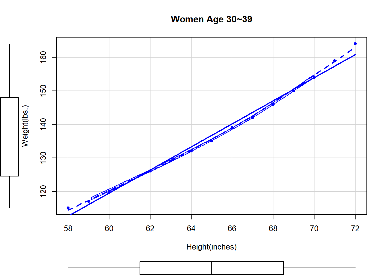
다중 회귀
require(MASS)
str(birthwt)
'data.frame': 189 obs. of 10 variables:
$ low : int 0 0 0 0 0 0 0 0 0 0 ...
$ age : int 19 33 20 21 18 21 22 17 29 26 ...
$ lwt : int 182 155 105 108 107 124 118 103 123 113 ...
$ race : int 2 3 1 1 1 3 1 3 1 1 ...
$ smoke: int 0 0 1 1 1 0 0 0 1 1 ...
$ ptl : int 0 0 0 0 0 0 0 0 0 0 ...
$ ht : int 0 0 0 0 0 0 0 0 0 0 ...
$ ui : int 1 0 0 1 1 0 0 0 0 0 ...
$ ftv : int 0 3 1 2 0 0 1 1 1 0 ...
$ bwt : int 2523 2551 2557 2594 2600 2622 2637 2637 2663 2665 ...# age(엄마의 나이), lwt(마지막 생리기간의 엄마의 몸무게), race(인종), smoke(임신 중 흡연상태), ptl(과거 조산 횟수), ht(고혈압의 기왕력), ui(uterine irritability 존재 여부)
out=lm(bwt~age+lwt+factor(race)+smoke+ptl+ht+ui,data=birthwt)
anova(out)Analysis of Variance Table
Response: bwt
Df Sum Sq Mean Sq F value Pr(>F)
age 1 815483 815483 1.9380 0.1656022
lwt 1 2967339 2967339 7.0519 0.0086284 **
factor(race) 2 4750632 2375316 5.6450 0.0041901 **
smoke 1 6291918 6291918 14.9529 0.0001538 ***
ptl 1 732501 732501 1.7408 0.1887130
ht 1 2852764 2852764 6.7796 0.0099900 **
ui 1 5817995 5817995 13.8266 0.0002676 ***
Residuals 180 75741025 420783
---
Signif. codes: 0 '***' 0.001 '**' 0.01 '*' 0.05 '.' 0.1 ' ' 1# coefplot 패키지를 이용하면 계수 플롯을 만들 수 있습니다.
# 신뢰구간이 0을 포함하지 않으면 통계적으로 유의하다고 볼 수 있습니다.
library(coefplot)Warning: package 'coefplot' was built under R version 4.3.2coefplot(out)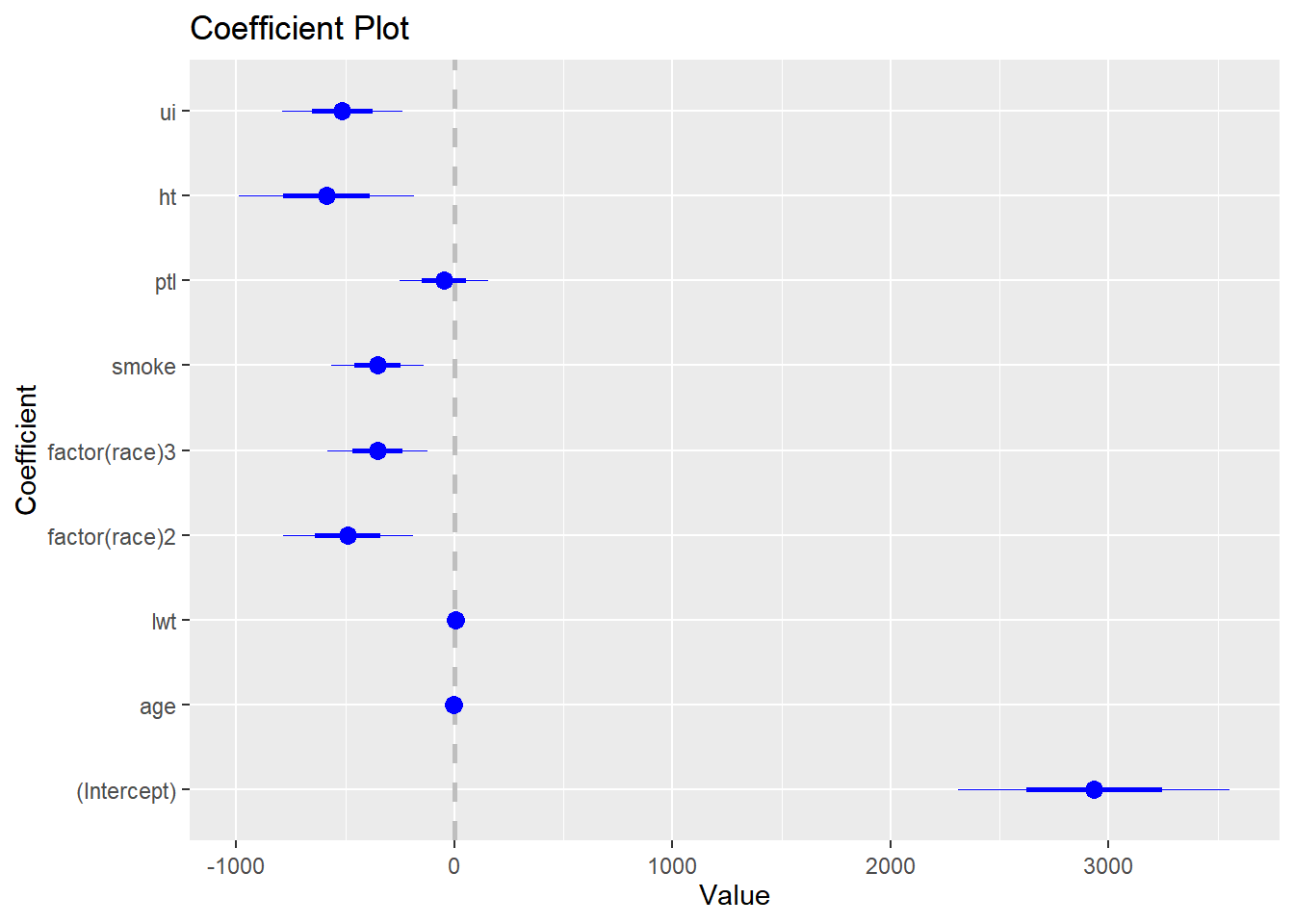
#분산분석표에서 age와 ptl에 유의하지 않으므로 두 변수를 제거한 모형을 만들고 두 변수의 중요도를 평가하기 위해 F-test를 실시합니다. F-test는 두 모형의 설명력을 비교하여 첫번째 모형에서 제거된 변수들의 기여도를 평가한다고 생각하면 됩니다. anova(작은모형, 큰모형)

out2=lm(bwt~lwt+factor(race)+smoke+ht+ui,data=birthwt)
anova(out2,out)
Analysis of Variance Table
Model 1: bwt ~ lwt + factor(race) + smoke + ht + ui
Model 2: bwt ~ age + lwt + factor(race) + smoke + ptl + ht + ui
Res.Df RSS Df Sum of Sq F Pr(>F)
1 182 75937505
2 180 75741025 2 196480 0.2335 0.792#F-test 결과 p-value가 0.792로 두 변수를 모두 제거할 수 있습니다.
anova(out2)Analysis of Variance Table
Response: bwt
Df Sum Sq Mean Sq F value Pr(>F)
lwt 1 3448639 3448639 8.2654 0.0045226 **
factor(race) 2 5076610 2538305 6.0836 0.0027701 **
smoke 1 6281818 6281818 15.0557 0.0001458 ***
ht 1 2871867 2871867 6.8830 0.0094402 **
ui 1 6353218 6353218 15.2268 0.0001341 ***
Residuals 182 75937505 417239
---
Signif. codes: 0 '***' 0.001 '**' 0.01 '*' 0.05 '.' 0.1 ' ' 1summary(out2)
Call:
lm(formula = bwt ~ lwt + factor(race) + smoke + ht + ui, data = birthwt)

Residuals:
     Min       1Q   Median       3Q      Max
-1842.14  -433.19    67.09   459.21  1631.03

Coefficients:
              Estimate Std. Error t value Pr(>|t|)
(Intercept)   2837.264    243.676  11.644  < 2e-16 ***
lwt              4.242      1.675   2.532 0.012198 *
factor(race)2 -475.058    145.603  -3.263 0.001318 **
factor(race)3 -348.150    112.361  -3.099 0.002254 **
smoke         -356.321    103.444  -3.445 0.000710 ***
ht            -585.193    199.644  -2.931 0.003810 **
ui            -525.524    134.675  -3.902 0.000134 ***
---
Signif. codes:  0 '***' 0.001 '**' 0.01 '*' 0.05 '.' 0.1 ' ' 1

Residual standard error: 645.9 on 182 degrees of freedom
Multiple R-squared:  0.2404,    Adjusted R-squared:  0.2154
F-statistic:   9.6 on 6 and 182 DF,  p-value: 3.601e-09
상호작용이 있는 다중 회귀
data(mtcars)
fit=lm(mpg~hp*wt, data=mtcars)
summary(fit)
Call:
lm(formula = mpg ~ hp * wt, data = mtcars)

Residuals:
    Min      1Q  Median      3Q     Max
-3.0632 -1.6491 -0.7362  1.4211  4.5513

Coefficients:
            Estimate Std. Error t value Pr(>|t|)
(Intercept) 49.80842    3.60516  13.816 5.01e-14 ***
hp          -0.12010    0.02470  -4.863 4.04e-05 ***
wt          -8.21662    1.26971  -6.471 5.20e-07 ***
hp:wt        0.02785    0.00742   3.753 0.000811 ***
---
Signif. codes:  0 '***' 0.001 '**' 0.01 '*' 0.05 '.' 0.1 ' ' 1

Residual standard error: 2.153 on 28 degrees of freedom
Multiple R-squared:  0.8848,    Adjusted R-squared:  0.8724
F-statistic: 71.66 on 3 and 28 DF, p-value: 2.981e-13plot(mpg~hp, data=mtcars, main="Interaction of hp:wt")
curve(31.41-0.06*x,add=TRUE)
curve(23.37-0.03*x,add=TRUE,lty=2,col=2)
curve(15.33-0.003*x,add=TRUE,lty=3,col=3)
legend("topright",c("2.2","3.2","4.2"),title="wt",lty=1:3,col=1:3)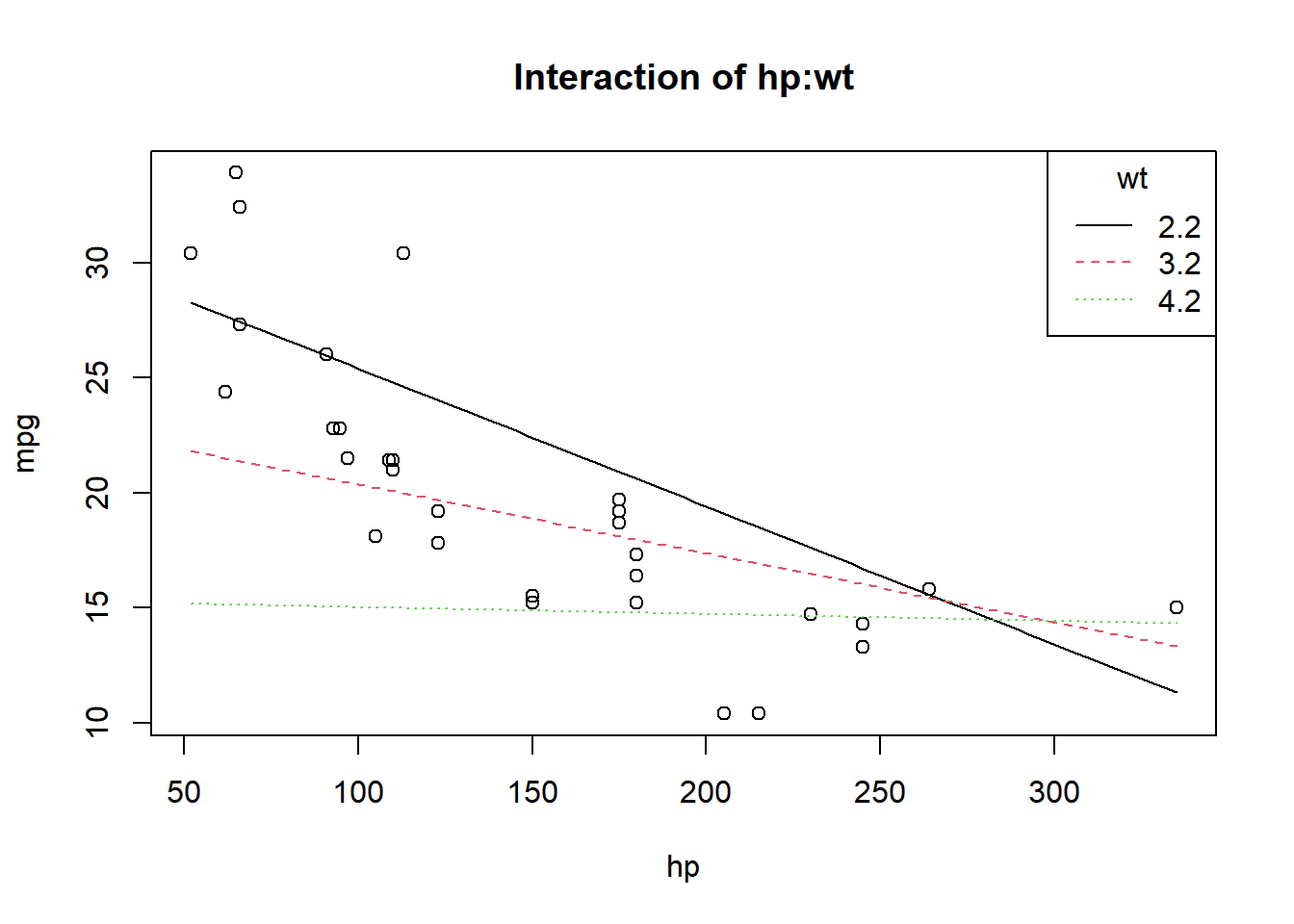
생존분석
rm(list=ls())
library(mombf)
Warning: package 'mombf' was built under R version 4.3.2Loading required package: mvtnormWarning: package 'mvtnorm' was built under R version 4.3.2Loading required package: ncvregWarning: package 'ncvreg' was built under R version 4.3.2Loading required package: mgcvWarning: package 'mgcv' was built under R version 4.3.2Loading required package: nlmeWarning: package 'nlme' was built under R version 4.3.2
Attaching package: 'nlme'The following object is masked from 'package:HistData':
WheatThe following object is masked from 'package:dplyr':
collapseThis is mgcv 1.9-0. For overview type 'help("mgcv-package")'.library(survival)
library(xtable)
Attaching package: 'xtable'The following objects are masked from 'package:Hmisc':
label, label<-library(ggplot2)
require(survival)
require(maxstat)Loading required package: maxstatWarning: package 'maxstat' was built under R version 4.3.2colon <- read.csv("colon.csv")
fit = survfit(Surv(time,status==1)~1, data=colon)
fitCall: survfit(formula = Surv(time, status == 1) ~ 1, data = colon)
n events median 0.95LCL 0.95UCL
[1,] 1858 920 2351 2018 2910#colon 데이터에서 time은 생존기간을 뜻하며 status가 1은 사망한 경우이고 0은 현재 살아있는 경우 입니다.
#Kaplan-Meier Curve 가운데 선이 KM curve이고 점선은 95% 신뢰구간입니다
plot(fit) # KM curve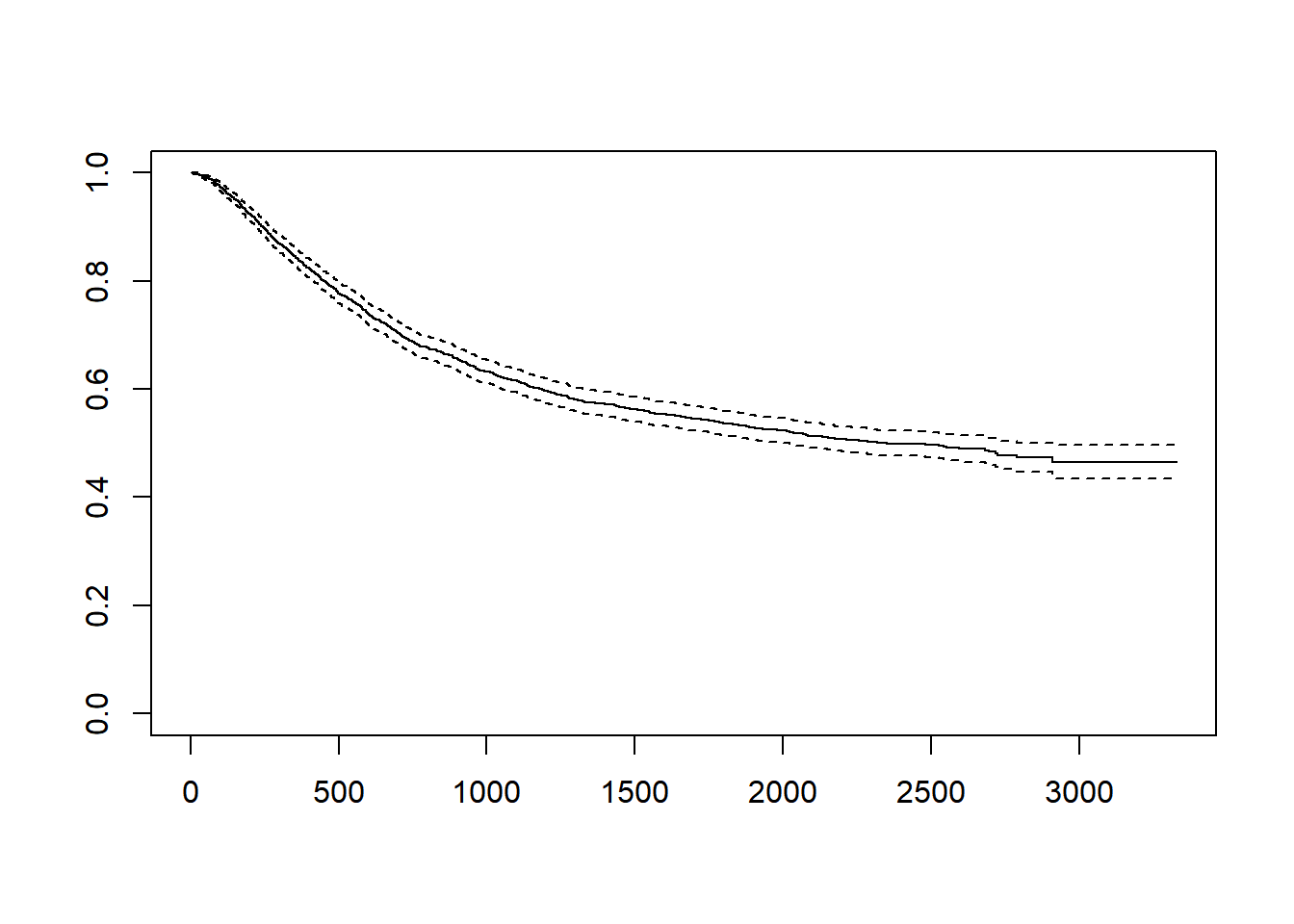
# rx열은 환자를 치료군에 따라 세군으로 나눈 데이터 입니다. 치료에 따른 생존율의 차이를 보기 위해서는 survfit 함수를 사용할때 “~rx”를 넣어줍니다.


fit1 = survfit(Surv(time,status==1)~rx,data=colon)
plot(fit1,col=1:3, lty=1:3)
legend("topright", legend=unique(colon$rx), col=1:3, lty=1:3)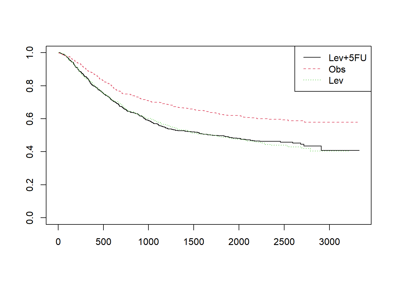
plot(fit1,col=1:3, lty=1:3, mark.time=TRUE)
legend("topright", legend=unique(colon$rx), col=1:3, lty=1:3)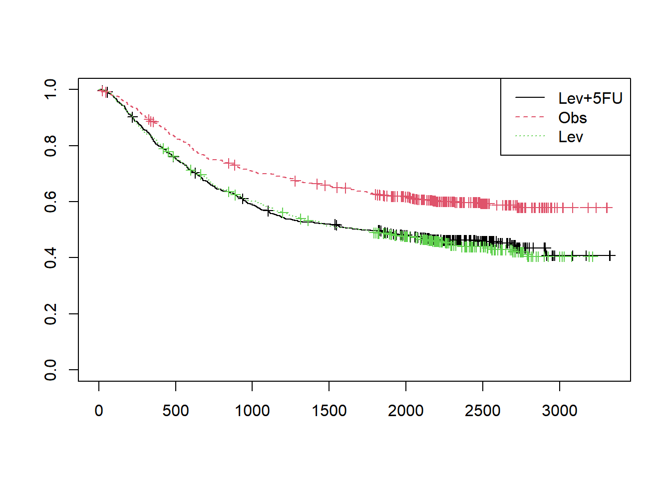
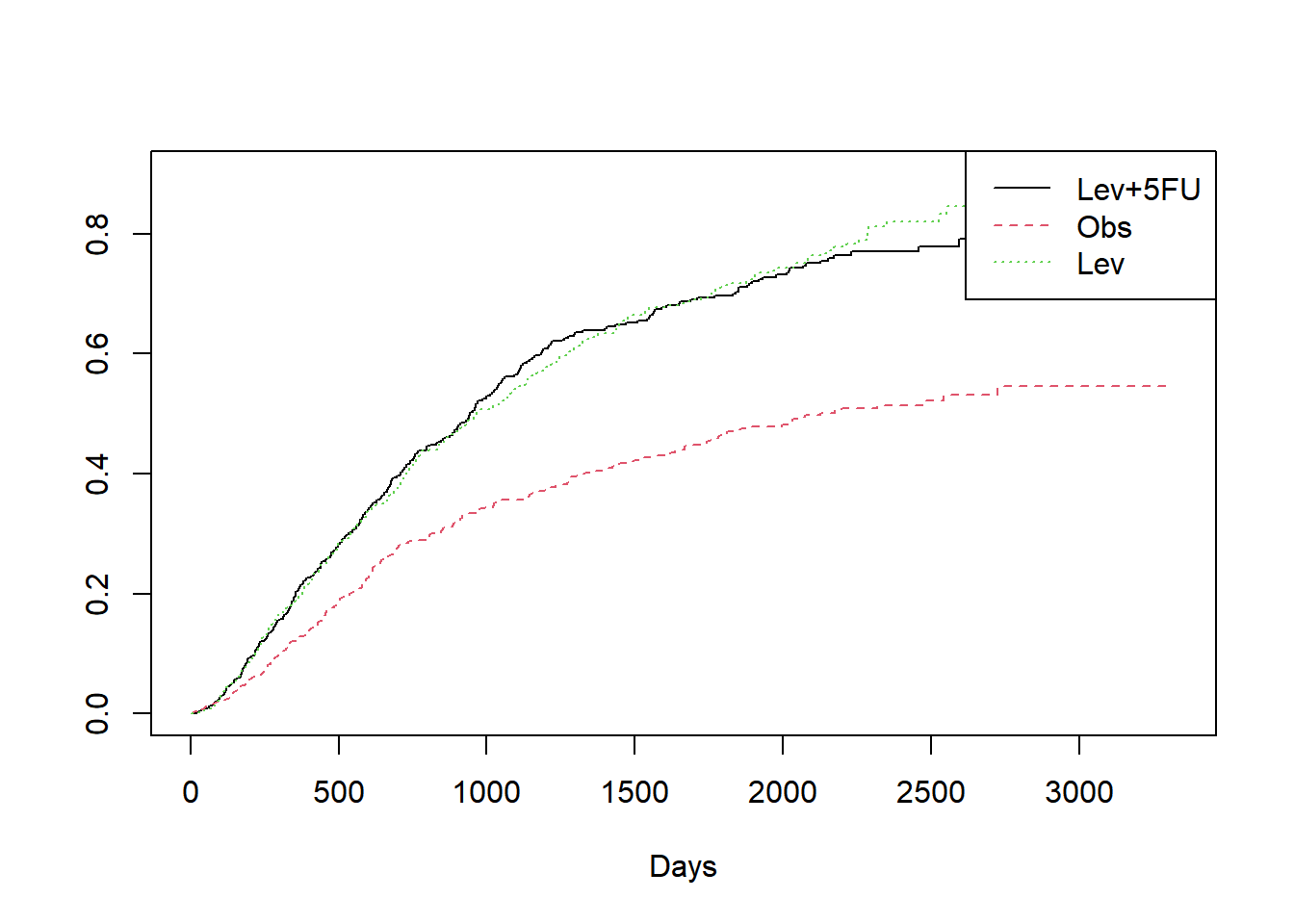
#누적함수 cumulative hazard
plot(fit1,col=1:3, lty=1:3, fun="cumhaz", xlab="Days")
legend("topright", legend=unique(colon$rx), col=1:3, lty=1:3)

require(GGally)
Loading required package: GGallyWarning: package 'GGally' was built under R version 4.3.2Registered S3 method overwritten by 'GGally':
method from
+.gg ggplot2fit = survfit(Surv(time,status==1)~rx, data=colon)
legend("topright", legend=unique(colon$rx), col=1:3, lty=1:3)