Code
RSI = 100 - \frac{100}{1 + RS}이 문서는 주요 암호화폐의 기술적 분석과 투자 전략을 다룹니다. 다양한 기술적 지표를 활용하여 투자 결정을 돕는 종합적인 분석을 제공합니다.
이동평균선은 다음 공식으로 계산됩니다: \(SMA_n = \frac{P_1 + P_2 + ... + P_n}{n}\)
RSI는 과매수/과매도 상태를 판단하는 지표입니다.
RSI = 100 - \frac{100}{1 + RS}여기서 RS는 상승평균/하락평균 입니다.
MACD는 단기와 장기 이동평균선의 차이를 보여주는 지표입니다.
MACD = EMA(12) - EMA(26)
Signal = EMA(9) \text{ of MACD}가격 변동성을 측정하는 지표입니다.
Upper Band = SMA(20) + 2 \times \sigma
Middle Band = SMA(20)
Lower Band = SMA(20) - 2 \times \sigma투자 점수는 다음과 같은 요소들을 고려하여 계산됩니다:
trend_score = mean(close > SMA50) * 3momentum_score = mean(RSI > 50 & RSI < 70) * 2volume_score = mean(volume > volume_ma) * 2volatility_score = (1 - volatility/max(volatility)) * 1.5bb_score = mean(close > BB_mid) * 1.5# 필요한 패키지 설치 및 로드
library(tidyverse)
library(tidyquant)
library(plotly)
library(TTR)
library(lubridate)
library(scales)
library(purrr)
# 분석할 코인 설정
coins <- c("BTC-KRW", "ETH-KRW", "XRP-KRW", "DOGE-KRW", "SHIB-KRW",
"SOL-KRW","USDT-KRW", "XLM-KRW" ) # Yahoo Finance 티커 형식
start_date <- "2020-01-01"
end_date <- Sys.Date()
# 코인 이름 매핑 함수 수정
get_coin_name <- function(symbol) {
# 입력값이 문자열인지 확인하고 처리
if (!is.character(symbol)) {
symbol <- deparse(substitute(symbol))
}
coin_names <- c(
"BTC-KRW" = "BTC/KRW - 비트코인",
"ETH-KRW" = "ETH/KRW - 이더리움",
"XRP-KRW" = "XRP/KRW - 리플",
"DOGE-KRW" = "DOGE/KRW - 도지코인",
"SHIB-KRW" = "SHIB/KRW - 시바이누",
"SOL-KRW" = "SOL/KRW - 솔라나",
"USDT-KRW" = "USDT/KRW - 테더",
"XLM-KRW" = "XLM/KRW - 스텔라루멘"
)
# 매핑된 이름이 없으면 원래 심볼 반환
result <- coin_names[symbol]
ifelse(is.na(result), as.character(symbol), result)
}
# 한국 화폐 단위 변환 함수 (소수점 지원)
korean_currency_format <- function(x) {
sapply(x, function(n) {
if (is.na(n)) return(NA)
if (n >= 1e8) { # 1억 이상
sprintf("%.1f억원", n/1e8)
} else if (n >= 1e4) { # 1만 이상
sprintf("%.1f만원", n/1e4)
} else if (n >= 1) { # 1원 이상
sprintf("%.0f원", round(n))
} else if (n >= 0.1) { # 0.1원 이상
sprintf("%.1f원", n)
} else if (n >= 0.01) { # 0.01원 이상
sprintf("%.2f원", n)
} else if (n >= 0.001) { # 0.001원 이상
sprintf("%.3f원", n)
} else if (n > 0) { # 0.001원 미만
sprintf("%.4g원", n) # 유효숫자 4자리로 표시
} else if (n == 0) { # 0원
"0원"
} else { # 음수
"-" + korean_currency_format(abs(n))
}
})
}
# 날짜 설정
start_date <- Sys.Date() - 365 # 1년 전부터
end_date <- Sys.Date() # 오늘까지
# 데이터 수집 및 전처리
crypto_data <- tq_get(coins,
from = start_date,
to = end_date,
get = "stock.prices") %>%
arrange(symbol,date) %>%
group_by(symbol) %>%
mutate(
display_name = get_coin_name(symbol),
# 이동평균선
SMA20 = TTR::SMA(close, n = 20),
SMA50 = TTR::SMA(close, n = 50),
SMA200 = TTR::SMA(close, n = 200),
# RSI
RSI = RSI(close, n = 14),
# MACD
MACD = MACD(close, nFast = 12, nSlow = 26, nSig = 9)[,'macd'],
Signal = MACD(close, nFast = 12, nSlow = 26, nSig = 9)[,'signal'],
# Bollinger Bands
BB_up = BBands(close, n = 20)[,'up'],
BB_mid = BBands(close, n = 20)[,'mavg'],
BB_down = BBands(close, n = 20)[,'dn'],
# 변동성
daily_returns = (close - lag(close))/lag(close),
volatility = rollapply(close, 20, function(x) sd(diff(log(x)))*sqrt(252)*100,
align = "right", fill = NA)
) %>%
ungroup()
# 이동평균선 계산 함수 정의
calculate_sma <- function(data, price_col, periods = c(20, 50, 200)) {
# 각 기간별 이동평균 계산
for (period in periods) {
col_name <- paste0("SMA", period)
data[[col_name]] <- TTR::SMA(data[[price_col]], n = period)
}
# NA 값을 이전 값으로 채우기
for (period in periods) {
col_name <- paste0("SMA", period)
data[[col_name]] <- if_else(is.na(data[[col_name]]),
lag(data[[col_name]], 1, default = first(na.omit(data[[col_name]]))),
data[[col_name]])
}
return(data)
}
# 데이터 수집 및 전처리
crypto_data <- tq_get(coins,
from = start_date,
to = end_date,
get = "stock.prices") %>%
arrange(symbol, date) %>%
group_by(symbol) %>%
filter(n() >= 20) %>% # 최소 20일치 데이터 필요
mutate(
display_name = get_coin_name(symbol)
) %>%
# 이동평균선 계산 함수 적용
group_modify(~calculate_sma(., "close")) %>%
mutate(
# RSI
RSI = TTR::RSI(close, n = 14),
# MACD
macd_data = TTR::MACD(close, nFast = 12, nSlow = 26, nSig = 9),
MACD = macd_data[,'macd'],
Signal = macd_data[,'signal'],
# Bollinger Bands
bb_data = TTR::BBands(close, n = 20),
BB_up = bb_data[,'up'],
BB_mid = bb_data[,'mavg'],
BB_down = bb_data[,'dn'],
# 변동성 및 수익률
daily_returns = (close/lag(close) - 1),
volatility = roll::roll_sd(daily_returns, width = 20) * sqrt(252) * 100
) %>%
# NA 값 처리
mutate(
across(c(RSI, MACD, Signal,
BB_up, BB_mid, BB_down, daily_returns, volatility),
~if_else(is.na(.), lag(., 1, default = first(na.omit(.))), .))
) %>%
ungroup() %>%
# 임시 컬럼 제거
select(-macd_data, -bb_data)
#
#
# # NA가 있는지 확인
# na_check <- sapply(crypto_data, function(x) sum(is.na(x)))
# print("NA 값 개수:")
# print(na_check[na_check > 0])
# 그래프 크기 조정을 위한 전역 옵션 설정
options(repr.plot.width = 12, repr.plot.height = 6)
# 가격 차트 시각화
price_charts <- crypto_data %>%
ggplot(aes(x = date, y = close, color = display_name)) +
geom_line() +
geom_line(aes(y = SMA20), linetype = "dashed", alpha = 0.5) +
geom_line(aes(y = SMA50), linetype = "dashed", alpha = 0.5) +
geom_line(aes(y = SMA200), linetype = "dashed", alpha = 0.5) +
facet_wrap(~display_name, scales = "free_y", ncol=4) +
labs(title = "Cryptocurrency Price Trends",
subtitle = "With 20, 50, and 200-day Moving Averages",
x = "Date",
y = "Price (KRW)") +
theme_minimal() +
#scale_y_log10(labels = scales::dollar_format()) +
scale_y_continuous(labels = korean_currency_format) + # log10 대신 continuous 사용
scale_color_brewer(palette = "Set1")+
theme(legend.position = "none")
# 볼린저 밴드 시각화
bollinger_charts <- crypto_data %>%
ggplot(aes(x = date)) +
geom_line(aes(y = close), color = "black") +
geom_line(aes(y = BB_up), color = "blue", linetype = "dashed") +
geom_line(aes(y = BB_down), color = "blue", linetype = "dashed") +
geom_ribbon(aes(ymin = BB_down, ymax = BB_up), fill = "blue", alpha = 0.1) +
facet_wrap(~display_name, scales = "free_y") +
labs(title = "Bollinger Bands Analysis",
x = "Date",
y = "Price (USD)") +
theme_minimal()
# RSI 시각화
rsi_charts <- crypto_data %>%
ggplot(aes(x = date, y = RSI, color = display_name)) +
geom_line() +
geom_hline(yintercept = c(30, 70), linetype = "dashed", color = "red") +
facet_wrap(~display_name) +
labs(title = "RSI Indicator",
subtitle = "With 30/70 Overbought/Oversold Levels",
x = "Date",
y = "RSI") +
theme_minimal()+
theme(legend.position = "none")
# 거래량 시각화
volume_charts <- crypto_data %>%
ggplot(aes(x = date, y = volume, fill = display_name)) +
geom_col(alpha = 0.7) +
facet_wrap(~display_name, scales = "free_y") +
labs(title = "Trading Volume Analysis",
x = "Date",
y = "Volume (USD)") +
theme_minimal() +
theme(legend.position = "none")+
scale_y_continuous(labels = korean_currency_format)
# 변동성 비교
volatility_comparison <- crypto_data %>%
ggplot(aes(x = date, y = volatility, color = display_name)) +
geom_line() +
facet_wrap(~display_name) +
labs(title = "Volatility Comparison",
subtitle = "30-Day Rolling Volatility",
x = "Date",
y = "Volatility (%)") +
theme(legend.position = "none")+
theme_minimal()
# 상관관계 분석
correlation_data <- crypto_data %>%
select(date, symbol, close) %>%
pivot_wider(names_from = symbol, values_from = close) %>%
select(-date) %>%
cor(use = "complete.obs")
correlation_plot <- correlation_data %>%
as.data.frame() %>%
rownames_to_column("Crypto1") %>%
pivot_longer(-Crypto1, names_to = "Crypto2", values_to = "Correlation") %>%
ggplot(aes(x = Crypto1, y = Crypto2, fill = Correlation)) +
geom_tile() +
scale_fill_gradient2(low = "red", high = "blue", mid = "white",
midpoint = 0, limit = c(-1,1)) +
geom_text(aes(label = round(Correlation, 2)), color = "black") +
labs(title = "Cryptocurrency Correlation Matrix") +
theme_minimal() +
theme(axis.text.x = element_text(angle = 45, hjust = 1))
# 요약 통계 계산
summary_stats <- crypto_data %>%
group_by(symbol) %>%
summarise(
Mean_Price = mean(close),
Median_Price = median(close),
SD_Price = sd(close),
Min_Price = min(close),
Max_Price = max(close),
Mean_Volume = mean(volume),
Mean_Volatility = mean(volatility, na.rm = TRUE),
Sharpe_Ratio = (mean(daily_returns, na.rm = TRUE) /
sd(daily_returns, na.rm = TRUE)) * sqrt(252)
) %>%
arrange(desc(Mean_Price)) %>%
mutate(across(where(is.numeric), round, 2))
# 성과 비교를 위한 정규화된 가격 차트
normalized_price_chart <- crypto_data %>%
group_by(symbol) %>%
mutate(normalized_price = (close / first(close)) * 100) %>%
ggplot(aes(x = date, y = normalized_price, color = display_name)) +
geom_line() +
labs(title = "Normalized Price Comparison",
subtitle = "Initial Price = 100",
x = "Date",
y = "Normalized Price") +
theme_minimal()
# investment_score 계산에도 적용
investment_score <- crypto_data %>%
group_by(symbol) %>%
summarise(
trend_score = mean(close > SMA50, na.rm = TRUE) * 3,
momentum_score = mean(RSI > 50 & RSI < 70, na.rm = TRUE) * 2,
volume_score = mean(volume > lag(SMA(volume, n = 20)), na.rm = TRUE) * 2,
volatility_score = (1 - mean(volatility, na.rm = TRUE) /
max(volatility, na.rm = TRUE)) * 1.5,
bb_score = mean(close > BB_mid, na.rm = TRUE) * 1.5,
recent_trend = mean(tail(daily_returns, 20) > 0, na.rm = TRUE) * 2,
total_score = trend_score + momentum_score + volume_score +
volatility_score + bb_score + recent_trend
) %>%
arrange(desc(total_score))
# 현재 상태 계산도 수정
current_status <- crypto_data %>%
group_by(symbol) %>%
mutate(volume_ma = SMA(volume, n = 20)) %>%
slice_tail(n = 1) %>%
select(symbol, close, RSI, volume, volume_ma, volatility) %>%
left_join(investment_score, by = "symbol")print(price_charts)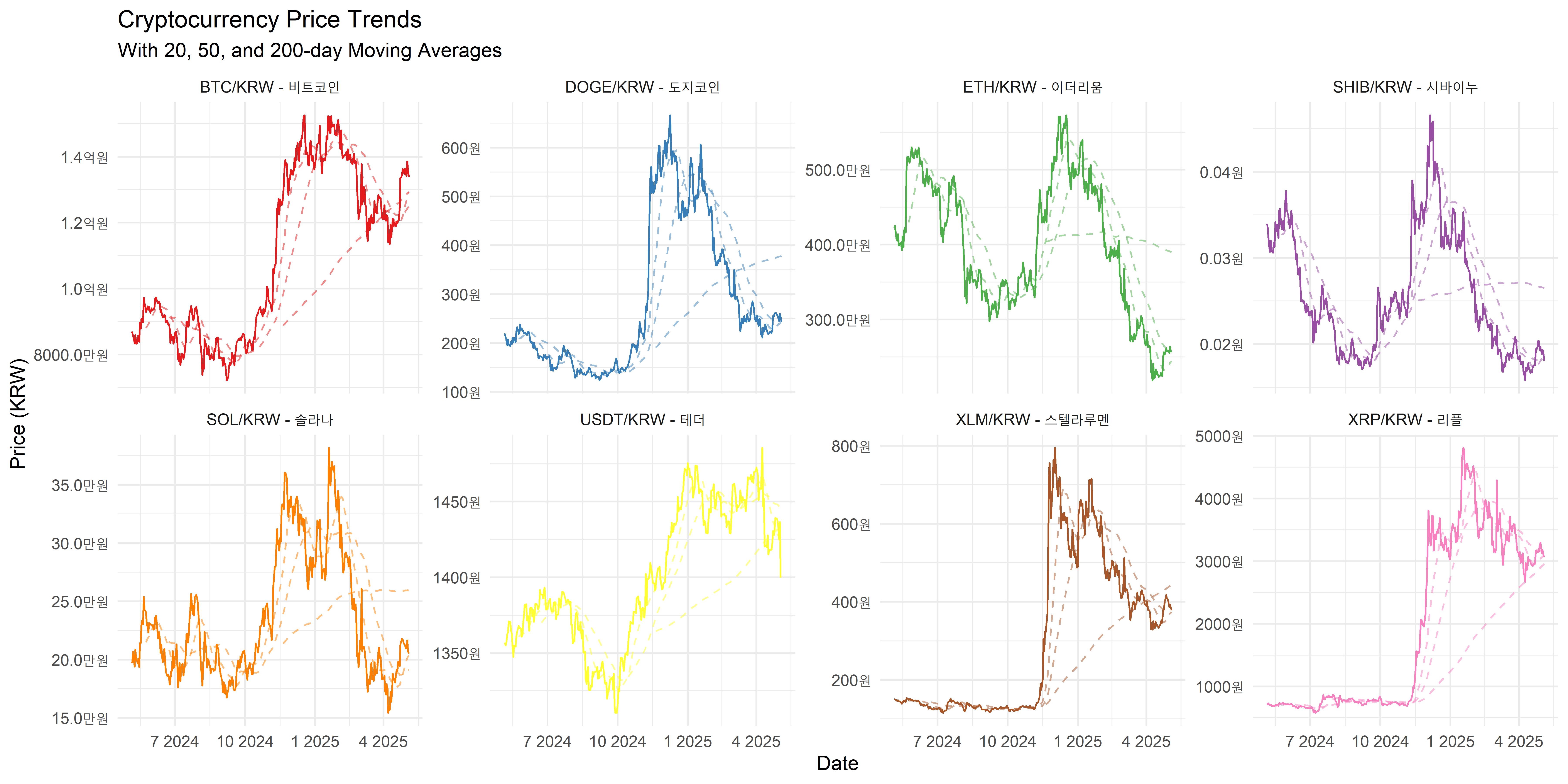
print(bollinger_charts)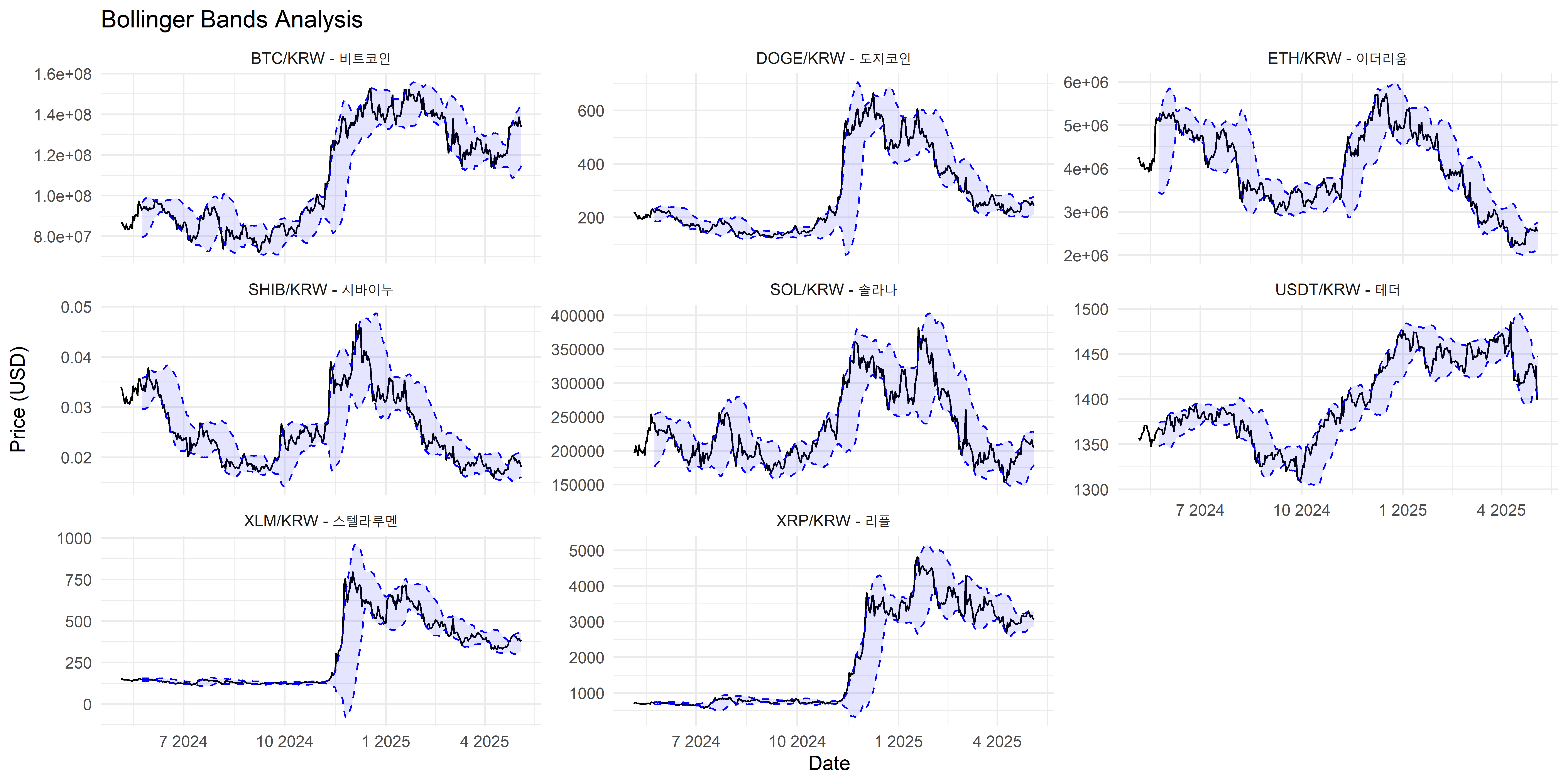
print(rsi_charts)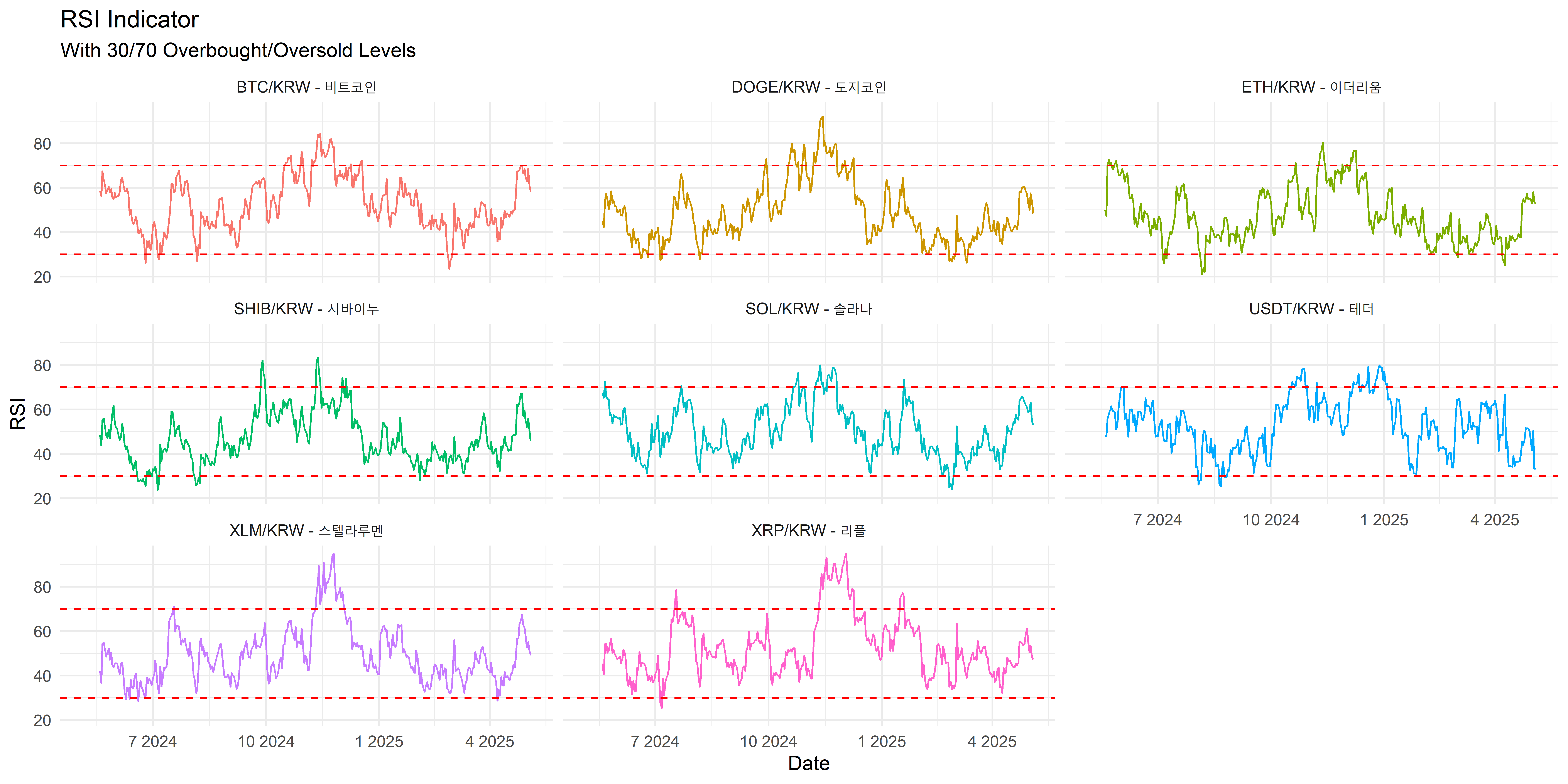
print(volume_charts)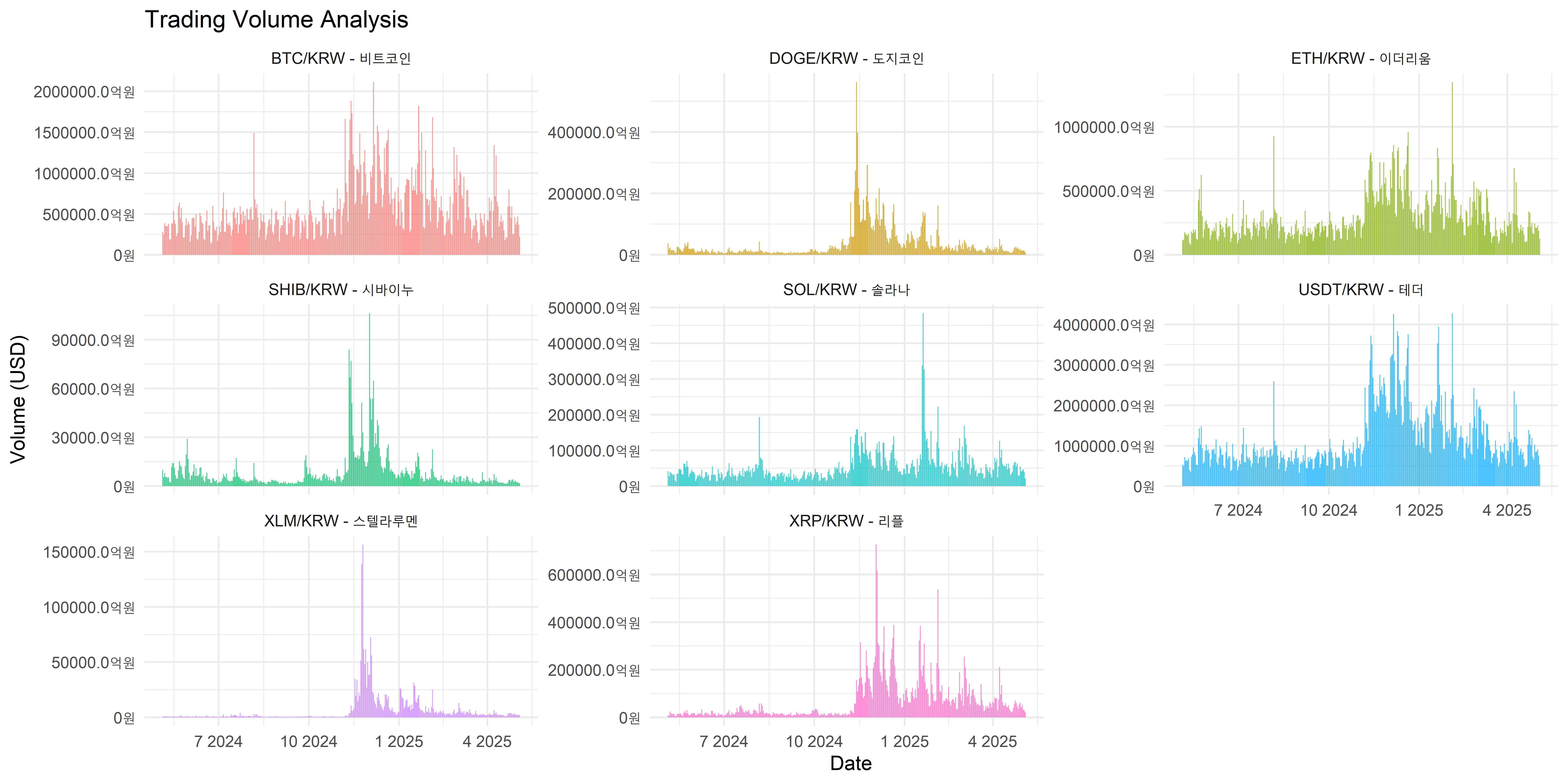
print(volatility_comparison)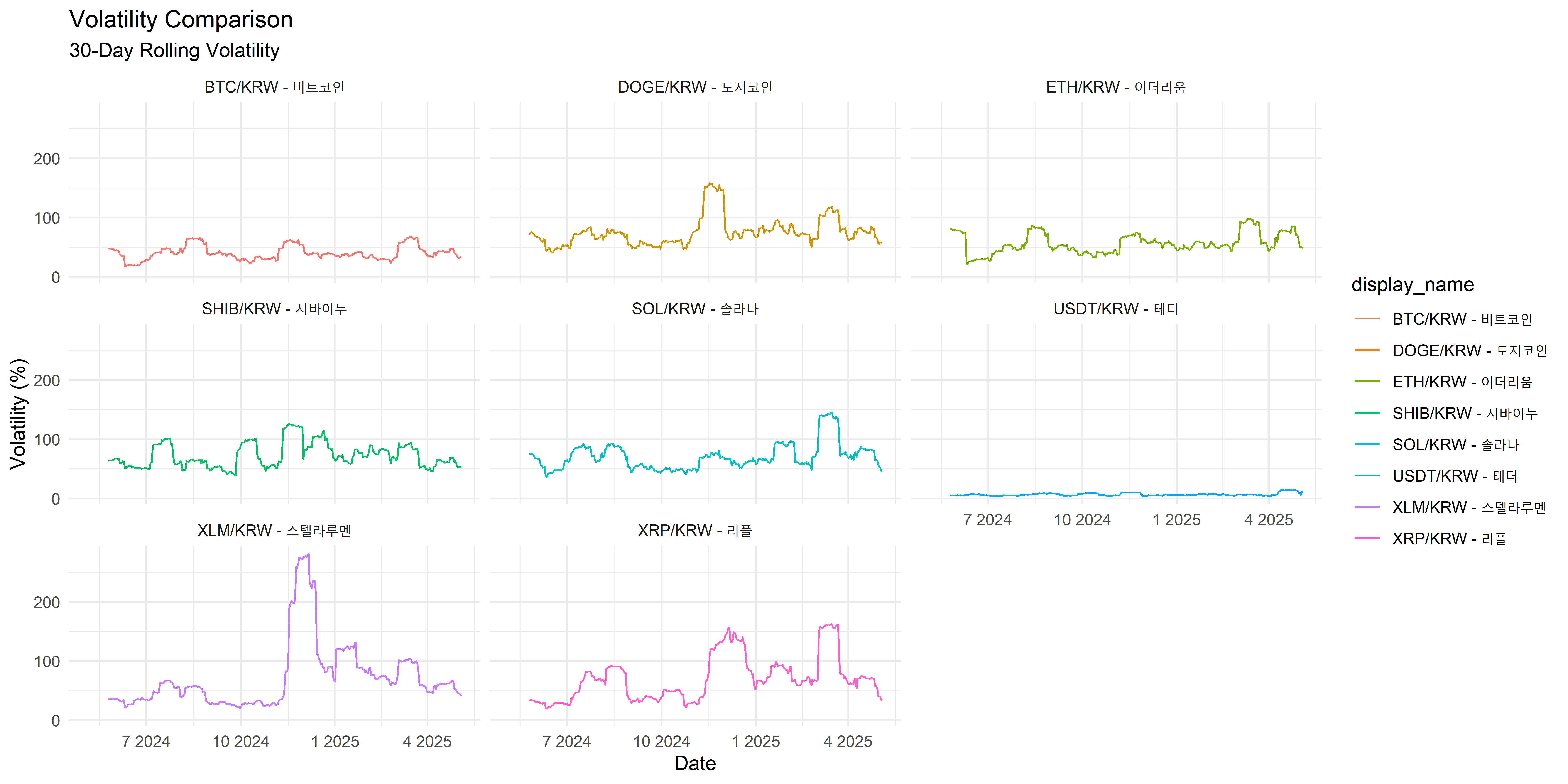
print(correlation_plot)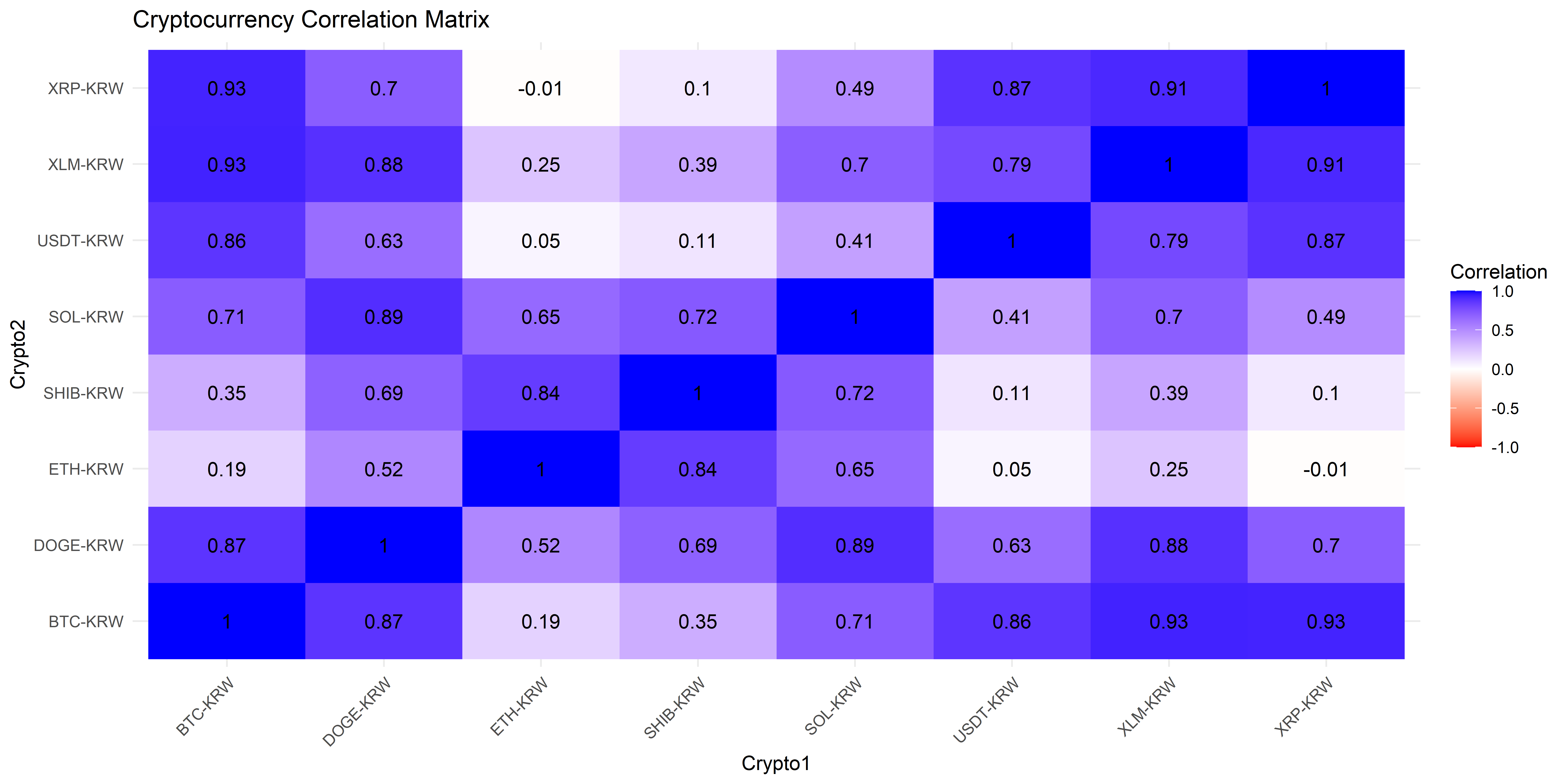
print(investment_score %>%
      select(symbol, total_score) %>%
      arrange(desc(total_score)))
# A tibble: 8 × 2
symbol total_score
<chr> <dbl>
1 USDT-KRW 6.35
2 BTC-KRW 5.94
3 XLM-KRW 5.61
4 XRP-KRW 5.60
5 SOL-KRW 5.46
6 DOGE-KRW 4.79
7 SHIB-KRW 4.63
8 ETH-KRW 4.60cat("\n=== 투자 전략 권장사항 ===\n")
=== 투자 전략 권장사항 ===top_picks <- investment_score %>%
slice_head(n = 3)
cat(sprintf("\n추천 투자 순위:\n"))
추천 투자 순위:for(i in 1:nrow(top_picks)) {
cat(sprintf("%d. %s (점수: %.2f)\n",
i,
top_picks$symbol [i],
top_picks$total_score[i]))
current_coin <- current_status %>%
filter(symbol == top_picks$symbol[i])
cat(sprintf(" 현재가: %s원\n RSI: %.2f\n 변동성: %.2f%%\n\n",
format(current_coin$close, big.mark=","),
current_coin$RSI,
current_coin$volatility))
}1. USDT-KRW (점수: 6.35)
   현재가: 1,400.067원
   RSI: 33.33
   변동성: 11.07%
2. BTC-KRW (점수: 5.94)
   현재가: 133,889,832원
   RSI: 58.11
   변동성: 32.97%
3. XLM-KRW (점수: 5.61)
   현재가: 378.5382원
   RSI: 49.17
변동성: 41.53%# 투자 전략 요약 출력
cat("\n=== 투자 전략 권장사항 ===\n")
=== 투자 전략 권장사항 ===top_picks <- investment_score %>%
slice_head(n = 3)
cat(sprintf("\n추천 투자 순위:\n"))
추천 투자 순위:for(i in 1:nrow(top_picks)) {
cat(sprintf("%d. %s (점수: %.2f)\n",
i,
top_picks$display_name[i], # display_name으로 변경
top_picks$total_score[i]))
current_coin <- current_status %>%
filter(symbol == top_picks$symbol[i])
cat(sprintf(" 현재가: %s원\n RSI: %.2f\n 변동성: %.2f%%\n\n",
format(current_coin$close, big.mark=","),
current_coin$RSI,
current_coin$volatility))
} 현재가: 1,400.067원
RSI: 33.33
변동성: 11.07% 현재가: 133,889,832원
RSI: 58.11
변동성: 32.97% 현재가: 378.5382원
RSI: 49.17
변동성: 41.53%# 투자 전략 제안 출력
cat("\n투자 전략 제안:\n")
투자 전략 제안:for(i in 1:nrow(top_picks)) {
coin_name <- top_picks$display_name[i] # display_name 사용
current <- current_status %>%
filter(symbol == top_picks$symbol[i])
cat(sprintf("\n%s:\n", coin_name)) # coin_name 사용
# RSI 기반 전략
if(current$RSI < 30) {
cat("- 과매도 구간으로 단기 반등 가능성 높음\n")
} else if(current$RSI > 70) {
cat("- 과매수 구간으로 단기 조정 가능성 있음\n")
} else {
cat("- RSI 중립구간으로 추가 모멘텀 관찰 필요\n")
}
# 거래량 기반 전략
if(current$volume > current$volume_ma) {
cat("- 거래량 증가로 추세 강화 신호\n")
} else {
cat("- 거래량 관망세로 신중한 접근 필요\n")
}
}- RSI 중립구간으로 추가 모멘텀 관찰 필요
- 거래량 관망세로 신중한 접근 필요- RSI 중립구간으로 추가 모멘텀 관찰 필요
- 거래량 관망세로 신중한 접근 필요- RSI 중립구간으로 추가 모멘텀 관찰 필요
- 거래량 관망세로 신중한 접근 필요cat("\n투자 주의사항:\n")
투자 주의사항:cat("* 위 분석은 기술적 지표만을 고려한 것으로, 실제 투자 시에는 펀더멘털 분석도 필요합니다.\n")* 위 분석은 기술적 지표만을 고려한 것으로, 실제 투자 시에는 펀더멘털 분석도 필요합니다.cat("* 암호화폐는 고위험 자산으로 분산 투자가 필수적입니다.\n")* 암호화폐는 고위험 자산으로 분산 투자가 필수적입니다.cat("* 투자 금액은 감당 가능한 수준으로 제한하시기 바랍니다.\n")* 투자 금액은 감당 가능한 수준으로 제한하시기 바랍니다.암호화폐 투자는 높은 수익 가능성과 함께 큰 리스크를 동반합니다. 본 분석의 기술적 지표들은 투자 결정을 보조하는 도구로 활용하되, 종합적인 분석과 리스크 관리가 필수적입니다.