Code
RSI = 100 - \frac{100}{1 + RS}이 문서는 미국 주요 기업들의 주가 기술적 분석과 투자 전략을 다룹니다. 다양한 기술적 지표를 활용하여 투자 결정을 돕는 종합적인 분석을 제공합니다.
이동평균선은 다음 공식으로 계산됩니다: \(SMA_n = \frac{P_1 + P_2 + ... + P_n}{n}\)
RSI는 과매수/과매도 상태를 판단하는 지표입니다.
RSI = 100 - \frac{100}{1 + RS}여기서 RS는 상승평균/하락평균 입니다.
# 필요한 패키지 설치 및 로드
library(tidyverse)
library(tidyquant)
library(plotly)
library(TTR)
library(lubridate)
library(scales)
library(purrr)

# 분석할 주식 설정
stocks <- c("AAPL", "MSFT", "GOOGL", "AMZN", "NVDA", "META", "TSLA", "JPM")
start_date <- Sys.Date() - 365  # 1년 전부터
end_date <- Sys.Date()          # 오늘까지

# 주식 이름 매핑 함수
get_stock_name <- function(symbol) {
  stock_names <- c(
    "AAPL" = "Apple Inc.",
    "MSFT" = "Microsoft Corp.",
    "GOOGL" = "Alphabet Inc.",
    "AMZN" = "Amazon.com Inc.",
    "NVDA" = "NVIDIA Corp.",
    "META" = "Meta Platforms Inc.",
    "TSLA" = "Tesla Inc.",
    "JPM" = "JPMorgan Chase & Co."
  )

  result <- stock_names[symbol]
  ifelse(is.na(result), as.character(symbol), result)
}

# 달러 통화 형식 함수
dollar_format_custom <- function(x) {
  scales::dollar_format(largest_with_cents = 1)(x)
}

# 데이터 수집 및 전처리
stock_data <- tq_get(stocks,
                    from = start_date,
                    to = end_date,
                    get = "stock.prices") %>%
  arrange(symbol, date) %>%
  group_by(symbol) %>%
  filter(n() >= 20) %>%  # 최소 20일치 데이터 필요
  mutate(
    display_name = get_stock_name(symbol),
    # 이동평균선
    SMA20 = TTR::SMA(close, n = 20),
    SMA50 = TTR::SMA(close, n = 50),
    SMA200 = TTR::SMA(close, n = 200),

    # RSI
    RSI = TTR::RSI(close, n = 14),

    # MACD
    macd_data = TTR::MACD(close, nFast = 12, nSlow = 26, nSig = 9),
    MACD = macd_data[,'macd'],
    Signal = macd_data[,'signal'],

    # Bollinger Bands
    bb_data = TTR::BBands(close, n = 20),
    BB_up = bb_data[,'up'],
    BB_mid = bb_data[,'mavg'],
    BB_down = bb_data[,'dn'],

    # 변동성 및 수익률
    daily_returns = (close/lag(close) - 1),
    volatility = roll::roll_sd(daily_returns, width = 20) * sqrt(252) * 100
  ) %>%
ungroup()# 가격 차트 시각화
price_charts <- stock_data %>%
ggplot(aes(x = date, y = close, color = display_name)) +
geom_line() +
geom_line(aes(y = SMA20), linetype = "dashed", alpha = 0.5) +
geom_line(aes(y = SMA50), linetype = "dashed", alpha = 0.5) +
geom_line(aes(y = SMA200), linetype = "dashed", alpha = 0.5) +
facet_wrap(~display_name, scales = "free_y", ncol=2) +
labs(title = "Stock Price Trends",
subtitle = "With 20, 50, and 200-day Moving Averages",
x = "Date",
y = "Price (USD)") +
theme_minimal() +
scale_y_continuous(labels = scales::dollar_format()) +
scale_color_brewer(palette = "Set1") +
theme(legend.position = "none")
print(price_charts)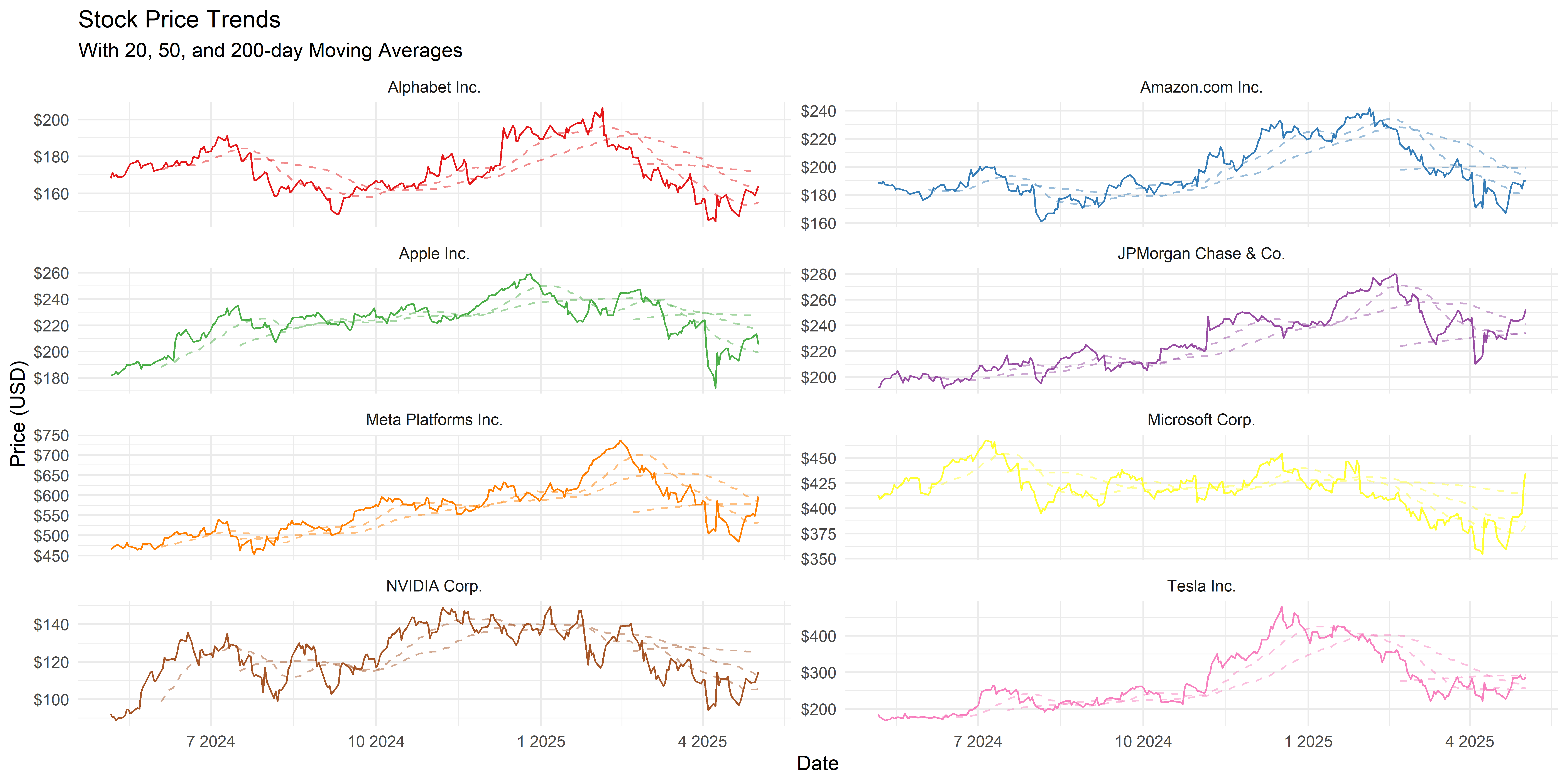
## 볼린저 밴드 분석
bollinger_charts <- stock_data %>%
  ggplot(aes(x = date)) +
  geom_line(aes(y = close), color = "black") +
  geom_line(aes(y = BB_up), color = "blue", linetype = "dashed") +
  geom_line(aes(y = BB_down), color = "blue", linetype = "dashed") +
  geom_ribbon(aes(ymin = BB_down, ymax = BB_up), fill = "blue", alpha = 0.1) +
  facet_wrap(~display_name, scales = "free_y", ncol=2) +
  labs(title = "Bollinger Bands Analysis",
       x = "Date",
       y = "Price (USD)") +
  theme_minimal() +
  scale_y_continuous(labels = scales::dollar_format())

print(bollinger_charts)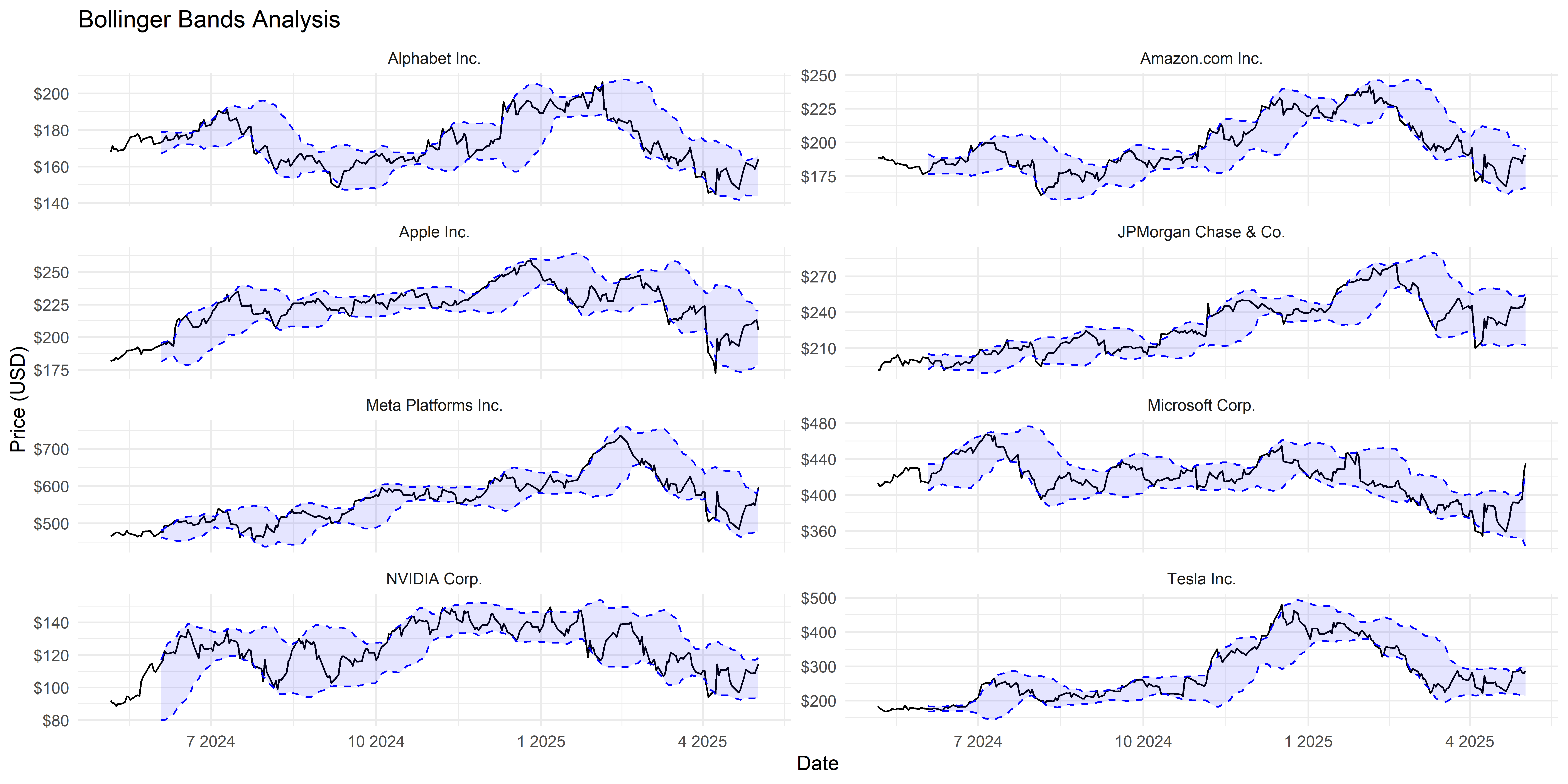
## RSI 분석
rsi_charts <- stock_data %>%
  ggplot(aes(x = date, y = RSI, color = display_name)) +
  geom_line() +
  geom_hline(yintercept = c(30, 70), linetype = "dashed", color = "red") +
  facet_wrap(~display_name, ncol=2) +
  labs(title = "RSI Indicator",
       subtitle = "With 30/70 Overbought/Oversold Levels",
       x = "Date",
       y = "RSI") +
  theme_minimal() +
  theme(legend.position = "none")

print(rsi_charts)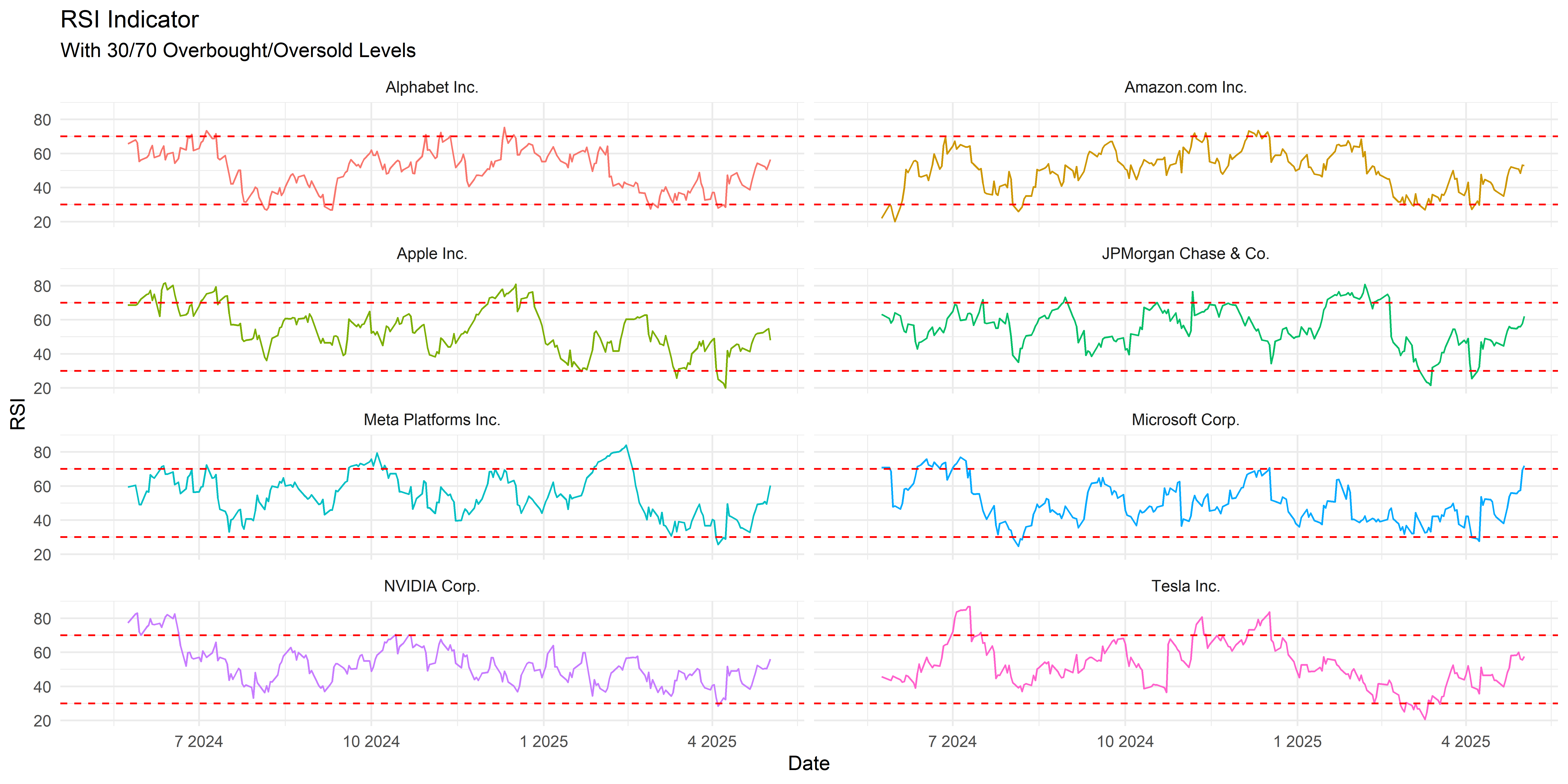
## 거래량 분석
volume_charts <- stock_data %>%
  ggplot(aes(x = date, y = volume/1e6, fill = display_name)) +
  geom_col(alpha = 0.7) +
  facet_wrap(~display_name, scales = "free_y", ncol=2) +
  labs(title = "Trading Volume Analysis",
       x = "Date",
       y = "Volume (Millions)") +
  theme_minimal() +
  theme(legend.position = "none")

print(volume_charts)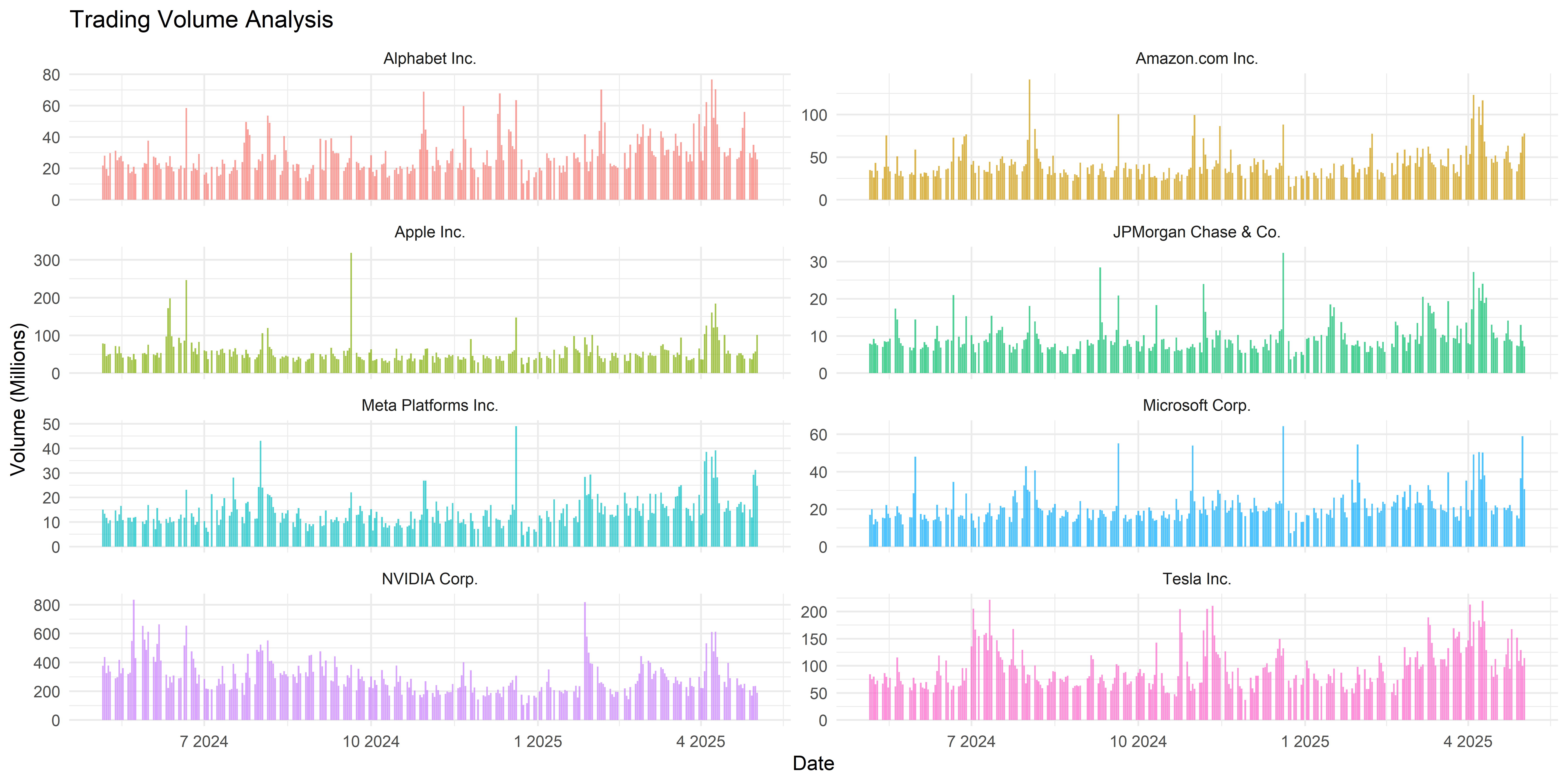
## 상관관계 분석
correlation_data <- stock_data %>%
  select(date, symbol, close) %>%
  pivot_wider(names_from = symbol, values_from = close) %>%
  select(-date) %>%
  cor(use = "complete.obs")

correlation_plot <- correlation_data %>%
  as.data.frame() %>%
  rownames_to_column("Stock1") %>%
  pivot_longer(-Stock1, names_to = "Stock2", values_to = "Correlation") %>%
  ggplot(aes(x = Stock1, y = Stock2, fill = Correlation)) +
  geom_tile() +
  scale_fill_gradient2(low = "red", high = "blue", mid = "white",
                      midpoint = 0, limit = c(-1,1)) +
  geom_text(aes(label = round(Correlation, 2)), color = "black") +
  labs(title = "Stock Correlation Matrix") +
  theme_minimal() +
  theme(axis.text.x = element_text(angle = 45, hjust = 1))

print(correlation_plot)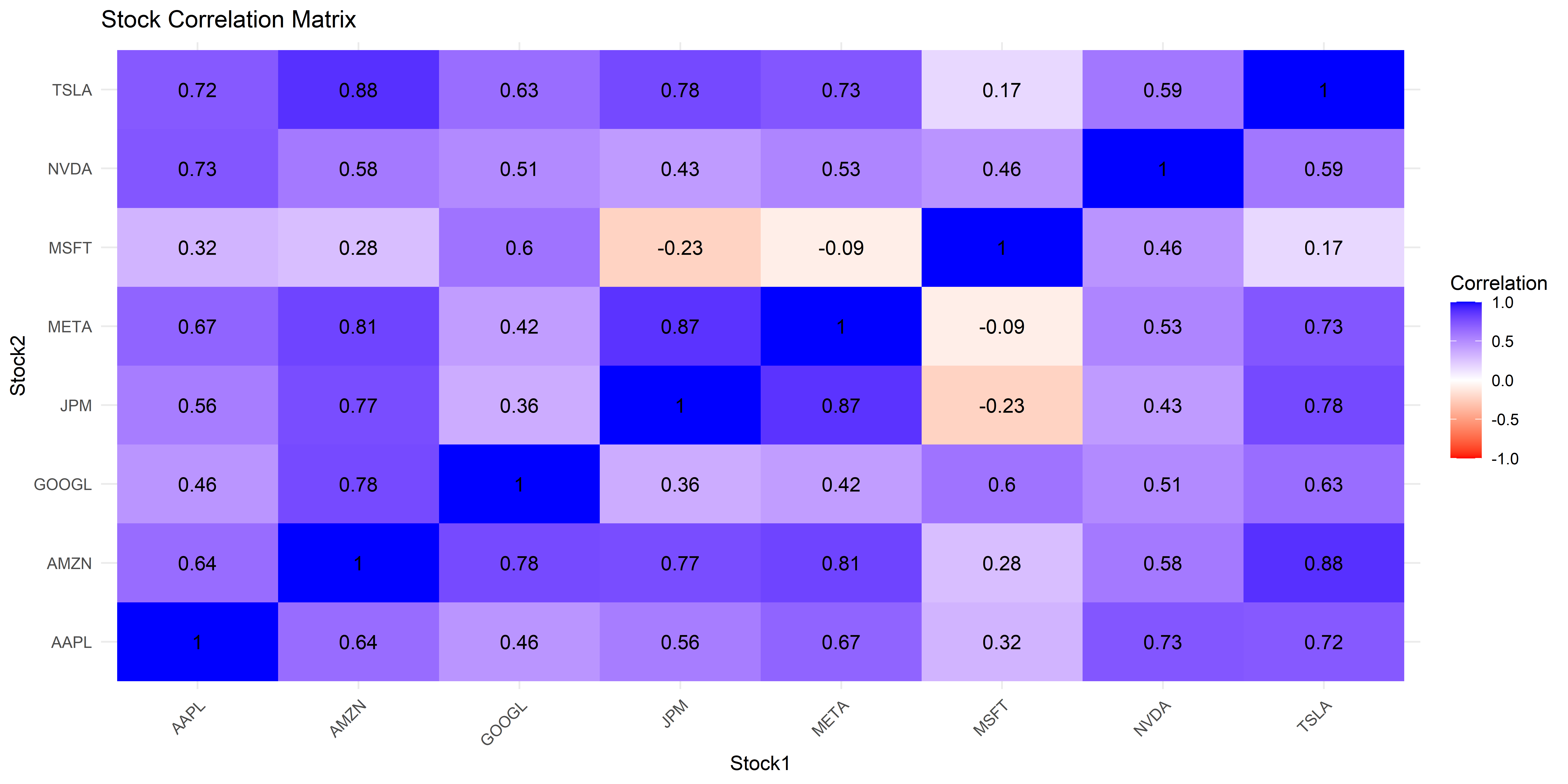
# 투자 점수 계산
investment_score <- stock_data %>%
  group_by(symbol) %>%
  summarise(
    # 추세 점수 (30%)
    trend_score = mean(close > SMA50, na.rm = TRUE) * 3,

    # 모멘텀 점수 (20%)
    momentum_score = mean(RSI > 50 & RSI < 70, na.rm = TRUE) * 2,

    # 거래량 점수 (20%)
    volume_score = mean(volume > lag(SMA(volume, n = 20)), na.rm = TRUE) * 2,

    # 변동성 점수 (15%)
    volatility_score = (1 - mean(volatility, na.rm = TRUE) /
                         max(volatility, na.rm = TRUE)) * 1.5,

    # 볼린저 밴드 점수 (15%)
    bb_score = mean(close > BB_mid, na.rm = TRUE) * 1.5,

    # 최근 추세 점수
    recent_trend = mean(tail(daily_returns, 20) > 0, na.rm = TRUE) * 2,

    # 총점 계산
    total_score = trend_score + momentum_score + volume_score +
      volatility_score + bb_score + recent_trend
  ) %>%
  arrange(desc(total_score))

# 현재 상태 계산
current_status <- stock_data %>%
  group_by(symbol) %>%
  mutate(volume_ma = SMA(volume, n = 20)) %>%
  slice_tail(n = 1) %>%
  select(symbol, display_name, close, RSI, volume, volume_ma, volatility) %>%
  left_join(investment_score, by = "symbol")

# 투자 점수 출력
print(investment_score %>%
      select(symbol, total_score) %>%
      arrange(desc(total_score)))
# A tibble: 8 × 2
symbol total_score
<chr> <dbl>
1 JPM 6.74
2 META 6.56
3 AAPL 6.31
4 TSLA 6.00
5 AMZN 5.94
6 GOOGL 5.60
7 NVDA 5.45
8 MSFT 4.96cat("\n=== 투자 전략 권장사항 ===\n")
=== 투자 전략 권장사항 ===top_picks <- investment_score %>%
slice_head(n = 3)
cat(sprintf("\n추천 투자 순위:\n"))
추천 투자 순위:for(i in 1:nrow(top_picks)) {
current_stock <- current_status %>%
filter(symbol == top_picks$symbol[i])
cat(sprintf("\n%d. %s (%s)\n",
i,
current_stock$display_name,
current_stock$symbol))
cat(sprintf(" 점수: %.2f\n", top_picks$total_score[i]))
cat(sprintf(" 현재가: $%.2f\n", current_stock$close))
cat(sprintf(" RSI: %.2f\n", current_stock$RSI))
cat(sprintf(" 변동성: %.2f%%\n", current_stock$volatility))
# 투자 전략 제안
cat("\n 투자 전략:\n")
# RSI 기반 전략
if(current_stock$RSI < 30) {
cat(" - 과매도 구간으로 단기 반등 가능성 높음\n")
} else if(current_stock$RSI > 70) {
cat(" - 과매수 구간으로 단기 조정 가능성 있음\n")
} else {
cat(" - RSI 중립구간으로 추세 따라 매매 전략 구사\n")
}
# 거래량 기반 전략
if(current_stock$volume > current_stock$volume_ma) {
cat(" - 거래량 증가로 현재 추세 강화 신호\n")
} else {
cat(" - 거래량 감소로 신중한 접근 필요\n")
}
}
1. JPMorgan Chase & Co. (JPM)
   점수: 6.74
   현재가: $252.51
   RSI: 62.12
   변동성: 49.23%

   투자 전략:
   - RSI 중립구간으로 추세 따라 매매 전략 구사
   - 거래량 감소로 신중한 접근 필요

2. Meta Platforms Inc. (META)
   점수: 6.56
   현재가: $597.02
   RSI: 60.39
   변동성: 72.62%

   투자 전략:
   - RSI 중립구간으로 추세 따라 매매 전략 구사
   - 거래량 증가로 현재 추세 강화 신호

3. Apple Inc. (AAPL)
   점수: 6.31
   현재가: $205.35
   RSI: 48.05
   변동성: 74.83%

   투자 전략:
   - RSI 중립구간으로 추세 따라 매매 전략 구사
- 거래량 증가로 현재 추세 강화 신호이 분석은 주요 미국 기업들의 기술적 분석을 기반으로 투자 전략을 제시합니다. 하지만 기술적 분석만으로는 완벽한 투자 판단을 내릴 수 없으며, 다음 요소들을 함께 고려해야 합니다:
투자자는 이러한 종합적인 분석을 바탕으로 자신의 투자 성향과 위험 감수 성향에 맞는 포트폴리오를 구성해야 합니다.